Wavelet Estimation of Kondratieff Waves: An Applica-tion to Long Cycles in Prices and World GDP

Abstract

In this paper we apply wavelet analysis to the detection of long waves in wholesale price index for France, the UK and the US because wavelets can easily overcome most of the methodological difficulties experienced in previ-ous methods.

The advantages of using wavelet multiresolution decomposition analysis for the analysis of long waves studied by Kondratieff are manifold: 1) long wave components are easily obtainable through multiresolution decomposition analysis; 2) no preliminary correction is needed; and 3) they can handily detect cycles that are not easily visible in trending series (as it is the case of the wholesale price index in the post-WWII period).

Comparisons with the chronology in the literature on long wave cycles for prices and with recent results for world GDP growth rates indicate that wavelet analysis can provide a reliable and useful statistical methodology in order to analyze the dynamics of long waves in historical time series.

Keywords: long wave cycles, wavelet analysis, wholesale prices, world GDP.

1. Introduction

After almost a century from its publication, Kondratieff's (1926) research on 50-year long cyclical movements in economic activity remains a fascinating, but still highly controversial theory (Bernard et al. 2014). Both the very presence and the driving forces and mechanisms generating such long waves are a matter of dispute. The very existence of long waves is questioned on the basis that available data are inadequate, since there are too few observations for rigorous test by means of spectral analysis. As to the working mechanism of the economy, the main dispute is over the adequacy of endogenous models based on intermittent clusters of technological innovations generated in the lead economy (hegemonic country) and diffused unevenly outwards to other economies through Schumpeter's (1939) ‘creative destruction’ process, with respect to exogenous models driven by external impulses such as wars (Goldstein 1988).¹

Still more controversial is the choice of the appropriate methodology for identification of long waves. The methods initially used for detecting long waves in economic variables aimed at isolating major fluctuations in the deviations of a variable around its trend through a combination of detrending procedures and smoothing techniques (Kondratieff 1926). These methods have been criticized for adopting ad-hoc solutions for trend estimation and moving average length, as well as for implying that trends and the fluctuations in the deviations from trends do not interact and influence each other (trend-cycle sepa-ration). In addition, statistical artifacts and significant errors in long waves detection can be created by, respectively, detrending methodologies and faulty trend estimates (see Freeman and Louçã 2001; Zarnovitz and Ozyildirim 2002). The similarity between detection of long waves and extraction of growth cycles² has favoured the application of spectral methods to long wave analysis.³

Although the spectral-theory approach seems to be a particularly appropriate method for long wave detection, application of spectral analysis has several drawbacks: the observed series need to be stationary in order to be analyzed with the tools of spectral analysis and, above all, long waves revealed by spectral analysis are based on the assumption of regular fixed periodicities. Both requirements are particularly troublesome as the dataset used in long waves analysis includes two hundred years of data influenced by several war episodes, especially the two WWs. In this paper we propose the application of a different statistical method for detecting long waves in economic variables that can easily overcome most of the methodological difficulties experienced in previous methods: wavelet analysis. Wavelets have ability to handle a variety of nonstationary and complex signals because their projections are local, rather than global. Moreover, the non-parametric nature of the multiresolution decomposition analysis is able to capture the irregular nature of the period and amplitude of economic cycles and captures cyclical processes with different durations. Specifically, we apply the multiresolution and energy decomposition analysis to price series for France, the UK and the US in order to be able to compare our findings with the evidence provided by early long wave authors on long waves patterns in prices. Moreover, we analyze whether long waves are a general phenomena by looking at cycles in economic activity for the world economy as a whole. Anticipating our results one can say that the long waves in prices and in world economic activity detected using wavelet analysis resemble the long wave chronologies reported in the literature by various authors. All in all, we believe that wavelet analysis can be considered as a reliable and useful statistical methodology for analyzing long wave patterns in economic variables.

The paper is organized as follows: Section 2 describes the main differences between spectral and wavelet analysis and briefly presents the main features and properties of wavelet analysis in comparison. Then, in Section 3 we apply the multiresolution and energy decomposition analysis to price series for France, the UK and the US so as to have long-wave patterns in prices comparable with the evidence provided by early long wave authors. Moreover, we analyze whether long waves are a general phenomenon by looking at cycles in economic activity for the world economy as a whole. Section 4 concludes the paper.

2. An Alternative Methodology for Long Waves Detection: Wavelet Analysis

The methodology for identification of long waves in aggregate economic time series is still a largely debated question in the literature on long-run patterns.

Starting from Kondratieff's methodology⁴ several alternative approaches have been used for long waves detection: moving average smoothing techniques, trend deviation, and phase period analysis (Goldstein 1988).

Each methodology used for identifying long wave cycles in economic time series depend on data pre-processing since data transformation is needed for features extraction.

However, the extraction of the cyclical component of interest rely on a number of specific ad hoc assumptions, such as the pre-definition of historical phase periods or the specification of a particular form for the secular trend (linear, quadratic, exponential, etc.) in estimating the trend component.

More recently, the long wave hypothesis has been tested by means of spectral analysis because of its ability to simultaneously break down any time series into a set of cyclical components having different frequencies (e.g., Kuczynski 1978; Van Ewijk 1982; Bieshaar and Kleinknecht 1984; Metz 1992, 2011; Reijnders 1990, 1992, 2009; Diebolt and Doliger 2006, 2008; Korotayev and Tsirel 2010).

2.1 Spectral vs Wavelet Analysis

Spectral analysis provides a frequency domain representation of a signal (or a function) where the same information as the original function is approximated by the sum of periodical functions with fixed frequencies, i.e. sines and cosines. The signal can then be analyzed for its frequency content because the Fourier coefficients of the transformed function represent the contribution of each sine and cosine function at each frequency.⁵

The simultaneous estimation of several cyclical components may be also pursued using wavelet analysis.⁶ Like spectral analysis, wavelet analysis allows to decompose any signal into a set of time scale components, each reflecting the evolution through time of the signal at a particular range of frequencies and to study the dynamics of each component separately, but with a resolution matched to its scale since the wavelet basis function is dilated (or compressed) according to a scale parameter to extract different frequency information. Moreover, the transformation to the frequency domain does not preserve the time information so that it is impossible to determine when a particular event took place, a feature that may be important in the analysis of economic relationships. In other words, it has only frequency resolution but not time resolution.

Both transforms can be viewed as a rotation in function space to a different domain which for Fourier Transform contains basis functions that are sines and cosines, whereas for the wavelet transform, this new domain contains more complex basis functions called wavelets (see Strang 1993). The basis functions used by the Fourier transform (upper and middle panel) and the wavelet transform (lower panel) are shown in Fig. 1.

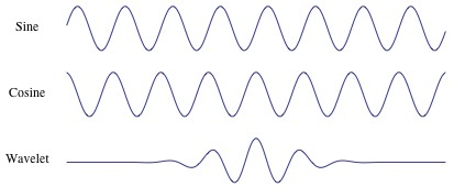
Fig. 1. Caption – Sines (top), cosines (middle) and wavelet (bottom) basis functions

Fig. 1 shows that wavelets are mathematical functions that transform the data into a mathematically equivalent representation by using a basis function that is similar to a sine and cosine function in that it also oscillates around zero, but differ because, as wavelets are constructed over finite intervals, they are well-localized both in the time and the frequency domain. Since the Fourier transform uses a linear combination of basis functions ranging over ± infinity, all projections in Fourier analysis are global, and thus a single disturbance affects all frequencies for the entire length of the series. Thus, if the signal is a non-periodic one, the summation of the periodic functions, sine and cosine, does not accurately represent the signal.

Such a feature restricts the usefulness of the Fourier transform to the analysis of stationary processes, whereas most economic and financial time series display frequency behavior that changes over time, i.e. they are nonstationary (Ramsey and Zhang 1996).

Hence, although spectral analysis is in principle an appropriate methodology for long wave analysis because of its ability to simultaneously estimate the contribution of several cyclical components, in practice its application is greatly limited by the requirement that the series is detrended in order to achieve stationarity. But then one is back in the realm of detrending methods along with their problems of arbitrariness in the estimation and elimination of the trend component.⁷

By contrast wavelet analysis may overcome the main problems evidenced by Fourier analysis since wavelets are compactly supported, as are all projections of a signal onto the wavelet space are essentially local, not global, and thus need not be homogeneous over time.

Being performed locally, the wavelet transform allows the analysis of series that by their nature, as it is for long historical time series data, are likely to exhibit short-lived transient components like abrupt changes, jumps, and volatility clustering, typical of war episodes or crisis episodes.

Unlike spectral analysis and related statistical techniques, wavelet analysis considers nonstationarity as an intrinsic property of the data rather than a problem to be solved by pre-processing the data.

Indeed, much of the usefulness of wavelet analysis has to do with its flexibility to handle a variety of complex and nonstationary signals so that the data need neither be detrended nor corrections for war years are needed anymore. Corrections for war periods (war data are influenced by pre-war armament booms, war economy and post-war reconstruction booms around WWII and to a lesser extent WWI) are generally applied to original data by interpolating series for the war years (Metz 1992) or a priori elimination of the impact of the war periods (Korotayev and Tsirel 2010) on the assumption that such shocks can be seen as disturbances in the normal structure of data.

Hence, with wavelet analysis we can avoid the practice of studying history by erasing part of the history (Freeman and Louçã 2001).

Finally, long waves revealed by spectral analysis are based on the assumption of regular fixed periodicities (van Duijn 1983), but if the signal is a nonperiodic one, the summation of the periodic functions like sines and cosines, does not accurately represent the signal.

By contrast wavelet analysis breaks down any time series into the sum of nonperiodic oscillatory components (quasi-periodic functions) whose irregular pattern is likely to resemble cyclical movements better than any approach requiring fixed periodicities.

All in all, wavelet analysis, as well as spectral analysis, is particularly well suited for detecting cycles, but unlike spectral methods has the ability to detect cyclical components that are spaced irregularly in time and can be applied to non-stationary time series.

2.2 Wavelet Analysis in Brief

In this subsection we briefly introduce the essential characteristics of wavelet analysis. Wavelets, their generation and their potential usefulness are discussed in intuitive terms in Ramsey (2010, 2014). A more technical exposition with many examples of the use of wavelets in a variety of fields is provided by Percival and Walden (2000), while an excellent introduction to wavelet analysis along with many interesting economic and financial examples is given in Gencay, Selcuk and Whitcher (2002) and Crowley (2007).

The wavelet transform maps a function f(t) from its original representation in the time domain into an alternative representation in the time-scale domain w(t, j) applying the transformation w(t, j) = ψ(.)f(t), where t is the time index, j – the scale (i.e. a specific frequency band) and ψ(.) – the wavelet filter. There are two basis wavelet filter functions: the father and the mother wavelets, φ and ψ, respectively. The first integrates to 1 and reconstructs the smooth and low frequency parts of a signal, whereas the latter integrates to zero and describes the detailed and high-frequency parts of a signal.

The formal definition of the father wavelet is the function

φ _J,k = 2^-(J/2) φ((t – 2^J k)/(2^J)) (1)

defined as non-zero over a finite time length support that corresponds to given mother wavelet

ψ _j,k = 2^-(j/2) ψ((t – 2^j k)/(2^j)) (2)

with j=1,.....,J in a J-level wavelets decomposition. The mother wavelet, as said above, plays a role similar to sines and cosines in the Fourier decomposition. It serves as a basis function to construct a set of wavelets, where each element in the wavelet set is obtained by compressing or dilating and shifting the mother wavelet, in order to approximate a signal.

For a discrete signal or function f₁, f₂, ...., f_n, the wavelet representation of the signal or function f(t) in L²(R) can be given by

f(t) = ∑_k s_J,kΦ_J,k(t) + ∑_k d_J,k Ψ_J,k(t) + … + ∑_k dj_,k Ψ_j,k(t) + … + ∑_k d_1,k Ψ1_,k(t), (3)

where J is the number of multiresolution components or scales, and k ranges from 1 to the number of coefficients in the specified components. The coefficients d_jk and s_Jk of the wavelet series approximations in (3) are the details and smooth wavelet transform coefficients representing, respectively, the projections of the time series onto the basic functions generated by the chosen family of wavelets, that is

d_j,k = ∫ ψ_j,k f(t)dt

s_J,k = ∫ φ_J,k f(t)dt

for j = 1, 2, ...., J. The smooth coefficients s_Jk mainly capture the underlying smooth behavior of the data at the coarsest scale, whereas details coefficients d_1k, …, d_jk, …, d_Jk, representing deviations from the smooth behaviour, provide progressively finer scale deviations.⁸

The multiresolution decomposition of the original signal f(t) is given by the following expression

f(t) =S_J + D_J + D_J–1 + ... + D_j + ... +D₁ , (4)

where S_J = ∑_k s_J,kΦ_J,k(t), and D_j = ∑_k d_J,k Ψ_J,k(t) with j=1,....,J. The sequence of terms S_J, D_J, ...D_j, ..., D₁ in (4) represent a set of components that provide representations of the signal at the different resolution levels 1 to J. The term S_J represents the smooth long-term component of the signal and the detail components D_j provide the increments at each individual scale, or resolution, level. Each signal component has a frequency domain interpretation. As the wavelet filter belongs to high-pass filter with passband given by the frequency interval [1/2^j+1, 1/2^j] for scales 1 < j < J, inverting the frequency range to produce a period of time we have that wavelet coefficients associated to scale j = 2 ^j–1 are associated to periods [2^j, 2^j+1].

The frequency domain interpretation of each signal component, in term of periods, is presented in Table 1 for a J = 5 level decomposition analysis.

Table 1. Frequency interpretation in periods for a J=5 level decomposition

Scale level J	Detail level Dj	Frequency resolution (years)
1	D1	2–4
2	D2	4–8
3	D3	8–16
4	D4	16–32
5	D5	32–64
6	S5	> 64

In addition to decompose a time series into several components each associated with a different resolution level, wavelets allow for an alternative representation of the variability of stochastic processes on a scale-by-scale basis through the energy decomposition analysis.

Let E be the total energy of a signal f(t) for j = 1, ..., J we have

E = E_J + ∑ _j=1^J E_{j ,}

where

E_J = ∑_k=1^n/2J s²_J,k

E_J = ∑_k=1^n/2j d²_J,k

are the energy of the scaling and wavelet coefficients, respectively. The expression shows that the total signal energy is the sum of the j^th level approximation signal and sum of all detail level signals 1^st detail to j^th detail. Indeed, since wavelet transform is an energy preserving transformation, the sum of the energies of the wavelet and the scaling coefficients is equal to the total energy of the data. In particular, by performing the energy decomposition analysis we can decompose the total energy of a series into the energy associated to each frequency component so as to detect which cyclical components contribute substantially more to the overall energy of the process relative to the others.

3. Nonparametric Estimation of Long Waves Using Wavelets

3.1 Long Waves in Prices

In this section we explore the usefulness of wavelet time scale decomposition analysis for the detection of long wave economic cycles similar to those discovered by Kondratieff in his original studies. Specifically, we investigate the presence of long waves in prices by examining the patterns in the wholesale price index for France, the UK and the US, the leading economies in the 18^th, 19^th and 20^th centuries, respectively, because these price series have provided the strongest supporting evidence for the long wave hypothesis by early 20^th century long wave investigators (e.g., van Gelderen 1913; Kondratieff 1926, 1935; de Wolff 1924; Schumpeter 1939).

Price data have been largely examined in the literature on long waves because prices have been for a long time the only economic data available and consistently measured, whereas output variables have been reconstructed by economic historians relatively recently and mostly back to the mid-19^th century. Moreover, since annual data on the wholesale price index go back to the late 18^th century, they allow using the longest possible time span as well as a number of observations higher than any corresponding international dataset on GDP whose data are only available from 1870 onwards only.

Finally, by using price indices data we can have direct evidence on the hypothesized changes in the long wave price behavior in the post-WWII period.

By using the discrete wavelet transform (DWT) we are able to decompose each price index into its different time scale components, each corresponding to a particular frequency band, and then to isolate the time scale component of interest.

We apply the maximal overlap discrete wavelet transform (MODWT) because the DWT has two main drawbacks: 1) the dyadic length requirement, i.e. a sample size divisible by 2^J; 2) the wavelet and scaling coefficients are not shift invariant, and, finally, the MODWT produces the same number of wavelet and scaling coefficients at each decomposition level as it does not use downsampling by two. In order to perform a wavelet analysis of a time series, a number of decisions must be made: which family of wavelet filters to use, what type of wavelet transform to apply, and how boundary conditions at the end of the series are to be handled. There are several families of wavelet filters available, such as Haar (discrete), symmlets and coiflets (symmetric), daublets (asymmetric), etc., differing by the characteristics of the transfer function of the filter and by filter lengths. Daubechies (1992) has developed a family of compactly supported wavelet filters of various lengths, the least asymmetric family of wavelet filters (LA), which is particularly useful in wavelet analysis of time series because it allows the most accurate alignment in time between wavelet coefficients at various scales and the original time series. With reflecting boundary conditions the original signal is reflected about its end point to produce a series of length 2N which has the same mean and variance as the original signal.

We apply the maximal overlap discrete wavelet transform (MODWT) to annual observations from 1791 to 2012 of the wholesale price indexes for France, the US and the UK , normalized to 100 for 1914, using the Daubechies least asymmetric (LA) wavelet filter of length L=8 based on eight non-zero coefficients (Daubechies 1992), with reflecting boundary conditions. The application of the MODWT with a number of levels (scales) J=5 to annual time series produces five wavelet details vectors D₁, D₂, D₃, D₄ and D₅ capturing oscillations with a period of 2–4, 4–8, 8–16, 16–32 and 32–64 years, respectively.

Given Kondratieff's definition of long wave cycles, that is cycles with a characteristic period from 40 to 60 years and with an average length of about 50 years (Kondratieff 1926, 1935), from the frequency domain interpretation of signal components provided in Table 1 we can identify which wavelet detail component closely corresponds to Kondratieff-type long wave cycles.

The D₅ detail component can provide an estimate of Kondratieff domain since its frequency range is between 32 and 64 years and its average cycle length is around 48 years.

Moreover, since no assumption has been made on the underlying nature of the signal and a criterion similar to a locally adaptive bandwidth has been adopted, the wavelet detail component D₅ represents a nonparametric estimation of a long cycle with average length equal to 48 years.

Since the MODWT is an energy (variance) preserving transform⁹ (Percival and Mofjeld 1997), it allows us to separate the contribution of energy in the price series due to changes at each time scale.

Specifically, the energy decomposition analysis allows us to separate the total energy of a series into the energy associated to each frequency component, and to detect the relative contribution of each cyclical component.

In particular, our specific interest is in measuring the relative importance of the component corresponding to the long waves as to all other cyclical components.

Fig. 2 shows three crystals energy related bar plots of the wholesale price series (net of the S₅ component) for France, the UK and the US from the energy decomposition analysis. Since for each wholesale price series most (or almost all) of the energy is concentrated in its large-scale features, with the small-scale features accounting for a very small fraction of the total variability, we apply the energy decomposition analysis to the raw series net of its long term smooth component S₅ in order to remove the overwhelming effects of S₅ components in the analysis. The result that longer cycle frequencies appear to carry most variability displays a striking similarity with the finding that Granger (1961) termed as ‘the typical spectral shape of an economic variable’ that shows how most of economic variables display a spectrum that exhibit a smooth declining shape with considerable power at very low frequencies.

The energy plots illustrate the distribution of the energy in the original signal at different scales and provide a measure of the relative importance of the various cycle types present in the price series.

There emerge two main findings: first, the residual energy at each scale level tends to decrease with the scale level, and second, most of this energy is concentrated at the detail level corresponding to the long wave component, D₅. This last result holds for the UK and the US, whereas in the case of France the level of energy at the D₄ level is slightly higher than that at the D₅ level.

On the whole, even if the total residual energy is modest, given the dominance of the S₅ components, we can conclude that the component corresponding to long waves provides the most significant contribution in terms of energy coefficients, especially in comparison to business cycles cyclical components.

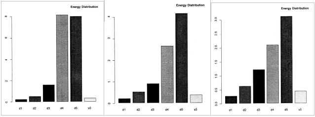
Fig. 2. Сaption – Energy decomposition analysis of wholesale price series (net of the S₅ component) for France (left), the UK (center) and the US (right)

The D₅ components of the wholesale price index for France, the UK and the US WPI_D5, are shown in Fig. 3, along with their corresponding raw series, WPI. Kondratieff's (1926) original chronology is reported using grey-shaded areas.

Five long waves in prices are clearly detected between 1790 and 2012 by means of wavelet multiresolution decomposition analysis (four and a half long waves are clearly detectable for France since the sample starting in 1803 captures the downswing phase of the first long wave).

Several features are worth mentioning from the visual inspection of the long waves presented in Fig. 3.

The main feature emerging from the visual inspection of long waves prices for all countries is the absence of regularities in terms of length and amplitude of such long wave patterns.

Indeed, these long wave patterns in wholesale price indexes are represented as an alternating sequence of historical phases of variable length.

Moreover, these long cycle movements in prices identified through wavelet multiresolution decomposition analysis are evident not only when the raw series is trendless, as it is in the pre-WWII period, but also after WWII when the trending behavior of the price level makes such long waves in price indexes hard to be detected.

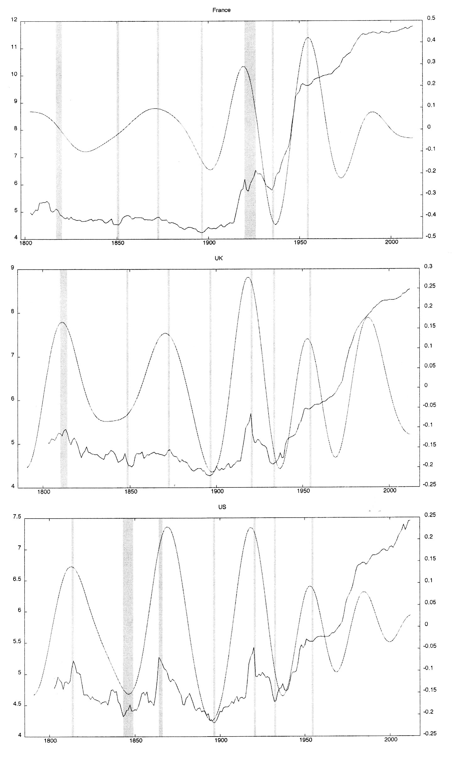
Fig. 3. Сaption – France (top), UK (middle) and US (bottom) wholesale price index along with its D₅ corresponding wavelet detail vector (smooth lines). Kondratieff's (1926) original chronology is indicated with grey-shaded areas.

A question highly debated in the literature is whether the wave pattern of price index dynamics has changed in the post-WWII period, because since then the wave pattern has ceased to be clearly traced in the price indices as a consequence of the strong positive trend of prices since the 1930s.

Our findings indicate that such a change after WWII has occurred for the US only, where a moderation in amplitude of the waves is evident by looking at the 4^th and 5^th price waves. Otherwise, for the UK there is no evidence of any reduction in the amplitude of long-term fluctuations in prices in the post-WWII period, whereas in the case of France the evidence shows that a considerable increase in the amplitude of price fluctuations is limited to those long waves taking place in the interwar and post-WWII periods.

Second, long movements in prices are closely related internationally, especially between the UK and the US. Long waves in UK and US wholesale prices are highly synchronized throughout the sample period, a finding that is consistent with the historical evidence on prices reported in the empirical literature for the major economies (see Goldstein 1988).

As regards France, although wholesale prices are out-of-phase with the UK and the US throughout the 19^th century, from the early 20^th century they are moving in phase. Such in-phase relationship holds throughout the 20^th century until the US wholesale price index begins moving out-of-phase as to the two European countries (see Figs. 1 and 2). Indeed, the diverging pattern emerging in the first decade of the new millennium indicates that a phase shift between the price waves of the US and those of the two European countries could have occurred.

After Kondratieff (1926) a huge number of long wave chronologies have been proposed by various authors, for example, Schumpeter (1939), Clark (1944), Dupriez (1947), Mandel (1975), Rostow (1978), van Duijn (1983), among the others. Hence, a natural question is to see how the dating scheme identified by the D₅ detail component accords with the consensus dates found in the literature.

In Table 2 peaks and troughs dates detected by the D₅ component are compared with turns in long waves of wholesale prices as reported in Burns and Mitchell (1946), as well as with overall chronologies reported in Kondratieff (1935) and Rostow (1978).¹⁰

Table 2. Peak and trough dates (in bold) of the D₅ component of wholesale prices for France, the UK and the US

	USA	UK	France	Kondratieff	Rostow
peak	1813	1812	–	1810–17	1815
	(1814)	(1813)
trough	1847	1835	1833	1844–51	1848
	(1843)	(1849)	(1851)
peak	1870	1870	1871	1870–75	1873
	(1864)	(1873)	(1872)
trough	1895	1898	1901	1890–96	1896
	(1896)	(1896)	(1896)
peak	1919	1919	1919	1914–20	1920
	(1920)	(1920)	(1926)
trough	1937	1937	1937	–	1935
	(1932)	(1933)	(1935)
peak	1954	1955	1955	–	1951
trough	1969	1970	1973	–	1972
peak	1985	1989	1990	–	–
trough	2000	–	–	–	–

Note: Long waves of wholesale prices as reported in Burns and Mitchell (1946) in parenthesis. Kondratieff's (1926) and Rostow's (1978) datings are reported in the last two columns.

With very few exceptions the dates of long wave phases detected by the D₅ detail component of the wholesale price index match closely with Burns and Mitchell's (1946) dates for individual countries. The main difference refers to the trough date in the mid-19^th century, which is anticipated to the early 1830s for France and the UK, although for the UK there is evidence of a prolonged period of low prices lasting until 1850, the consensus date for the trough of the downswing phase. A minor difference for France is also evident at the turn of the 19^th century where the trough is slightly delayed of a few years. Despite such minor differences in dating particular turning points, the overall dating scheme provided by wavelet decomposition analysis shows a close correspondence with Kondratieff's (1926) turning zones and Rostow's (1978) chronology. Interestingly, as evidenced by the comparison with Rostow's base dating scheme, such a correspondence holds not only for the pre-WWII period, but also after WWII, a period in which any evidence whatsoever on long waves in prices is difficult to identify because of the positive trend displayed by prices.

3.2. Long Waves in World GDP Growth Rates

A question highly debated in the literature on long cycles is whether long waves are only ‘price waves’ or such long term fluctuations exist also in production series and 'real' variables like industrial output, GDP, etc.

In other words, are these price movements simply a monetary phenomenon or are they reflecting long waves in overall economic activity? Although prices have proven very useful for detecting wave patterns in the early stages of the research on the presence of long waves, the trending behavior of wholesale prices after WWII has made long-term price fluctuations hard to detect.¹¹

As a result long waves scholars have shifted their attention away from price indices to world GDP dynamics taking advantage of the international datasets provided by Maddison (1995, 2001, 2003, 2009). Such a shift is based on the assumption, suggested by the first generation of long wave authors, that prices and production have the tendency to move together in the long term.¹²

On the theoretical side, the emphasis on economic growth follows, for example, from innovation theories like Schumpeter's (1939) theory of economic development, where long economic cycles are induced by ‘clusters of innovations’ originating from the innovating economy and spreading to followers countries. Hence, long economic cycles are explained by very important innovations or general-purpose technologies (Kriedel 2006) that imply the emergence of long waves of economic growth in world production dynamics.

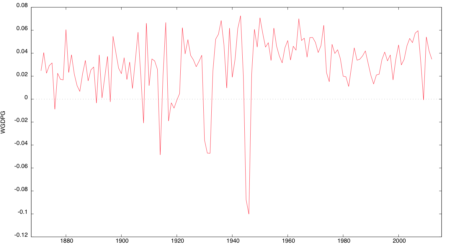
Fig. 4. Caption – World GDP Annual Growth Rates, 1871–2012

Following Lewis (1978), Kuczynski (1978), van Duijn (1983), Chase-Dunn and Grimes (1995) and, more recently, Korotayev and Tsirel (2010), we investigate the long wave pattern in World production dynamics using annual GDP growth rates between 1871 and 2012 (the World GDP growth rate series is shown in Fig. 5).¹³

In the top panel of Fig. 5 we show the D₅ component of the annual World GDP growth rate for the period from 1870 to 2012. To check for the robustness of the wave pattern detected by wavelet decomposition analysis in the bottom panel of Fig. 5 we show the wave pattern of the world GDP dynamics reported in Korotayev and Tsirel (2010: 24, Fig. 7) using spectral analysis and LOWESS.¹⁴

The phase dating of the D₅ component in world GDP growth rates shows a striking correspondence with Korotayev and Tsirel's (2010) chronology. Indeed, the overall long-wave pattern of the D₅ component is remarkably similar to the estimated wave pattern of world GDP dynamics, except in the 1920s, where the D₅ component shows a temporary increase before the 1929 financial crisis due to the strong economic upswing in Germany and Japan consequent to the pre-armament boom.

The sequence of upswings and downswings in world GDP growth rates in Fig. 5 delineates the historical long-wave pattern in world system dynamics during the last two centuries. In contrast to long-term fluctuations in prices dynamics, long wave patterns in the world economic dynamics provides evidence of only four long waves, each characterized by the creation and diffusion of general purpose technologies fuelling and propelling development and economic growth:

– the second¹⁵ wave (railway and steel industries) is visible only in the downswing phase from the 1870s to 1884, a period in which the world economy experiences a great depression;

– the third wave (chemical and electrical industries) combines a long wave upswing between 1884 and 1902, and the following long decline between the early 20^th century and the end of WWII (from 1903 to 1943), interrupted in the ‘golden 1920s’ by a temporary upswing, interpretable in terms of a reconstruction boom after WWI and the Germany and Japan's pre-war armament boom, which ended with the Great Depression;

– the fourth wave (petrochemicals and automobiles industries) combines the post-war growth upswing phase period between 1944 and 1963, and the downswing phase from 1964 to 1986. The first is characterized by the reconstruction effect of the mid-1940s and 1950s along with the ‘economic miracle’ in the European countries, the latter by class struggles and structural adjustments;

– the fifth wave (information, telecommunication and microelectronic industries), based on information technology, is currently under scrutiny in order to understand whether the recent financial crisis and the Great economic recession can represent the onset of a long downswing period following the upswing phase lasting since the late 1980s.

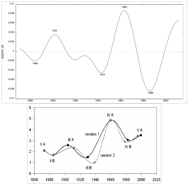
Fig. 5. Caption – Long waves for World GDP: D₅ (top panel) vs Korotayev and Tsirel (2010) (bottom panel)

3.3 Are Long Waves in Prices and Real Variables Similar?

Although the evidence provided by the early 20^th century long wave authors on the existence of long waves in the dynamics of the economy is based on the observation of long wave patterns in price series, many authors have later questioned this relation arguing that long wave patterns in prices do not correspond with the long-term movements of real variables (e.g., van Duijn 1983; Goldstein 1988). In particular, according to van Duijn (1983) institutional and market changes¹⁶ are likely to have weakened the relationship between price changes and production changes by affecting the mechanism of price formation, as evidenced by the uninterrupted increase of prices after the 1930s.

The results of the previous sections allow us analyzing whether these long-term movements in prices and economic growth are synchronous or not. Table 3 shows the long wave turning points for prices and economic growth as detected in Sections 2 and 3.¹⁷

Two main results are worth noting. First of all, as expected, the timing of these long cycles in prices and output is markedly different. There is no evidence of any synchronicity between the chronologies of price and production waves, nor before neither after the 1930s.

Second, as to the lead/lag relationship between production and prices, the evidence provided by Goldstein (1988), with production leading prices by a value close to 10–15 years, is confirmed only for the pre-1930s period. Indeed, after the 1930s the timing relationship between production and prices seems to reverse, with the turning points in prices leading those in production by a number of years that is gradually increasing over time.

Table 3. Long waves chronologies in production and prices

	Production	Prices
peak	–	1873
trough	1885	1896
peak	1902	1920
trough	1944	1935
peak	1964	1951
trough	1987	1972
peak	–	1988

4. Conclusions

In this paper we propose the application of wavelet analysis to detect long waves of the type examined by Kondratieff in the 1920s. The usefulness and reliability of wavelets for analyzing long wave patterns in economic variables has been tested by applying wavelet multiresolution and energy decomposition analysis to price and production series examined in the previous literature by many authors.

The advantages shown by wavelet multiresolution decomposition analysis for the analysis of long waves studied by Kondratieff are manifold:

– in contrast to other methodologies estimating simultaneously several cyclical components, wavelets, being a local transform, are constructed over finite intervals of time. As a consequence, no preliminary detrending procedure is needed anymore, as well as any correction for war periods;

– the outcome is represented by non-periodic cycles, that is oscillations are not regular in the timing and duration of upswings and downswings;

– they can handily detect cycles that are not easily visible in trending series (as it is the case of the wholesale price index in the post-WWII period).

All in all, we believe that wavelet analysis, because of its ability to deal with stationary and non-stationary series, can easily overcome most of the methodological difficulties faced by previous methods and can provide a unifying framework for analyzing the dynamics of long waves in historical economic and financial variables.

References

Bernard L., Gevorkyan A., Palley T., and Semmler W. 2014. Time Scales and Mechanisms of Economic Cycles: A Review of Theories of Long Waves. Review of Keynesian Economics 2 (1): 87–107.

Bieshaar H., and Kleinknecht A. 1984. Kondratieff Long Waves in Aggregate Output? An Econometric Test. Konjunkturpolitik 30(5): 279–303.

Burns A. F., and Mitchell W. C. 1946. Cyclical Changes in Cyclical Behavior. Measuring Business Cycles. NBER / Ed. by A. F. Burns, and W. C. Mitchell, pp. 424–471. New York: NBER.

Chase-Dunn C., and Grimes P. 1995. World-Systems Analysis. Annual Review of Sociology 21: 387–417.

Clark C. 1944. The Economics of 1960. London: MacMillan.

Crowley P. 2007. A Guide to Wavelets for Economists. Journal of Economic Surveys 21: 207–267.

Daubechies I. 1992. Ten Lectures on Wavelets. CBSM-NSF Regional Conference Series in Applied Mathematics. Vol. 61. SIAM, Philadelphia: SIAM (Society for Industrial and Applied Mathematics).

Diebolt C., and Doliger C. 2006. Economic Cycles under Test: A Spectral Analysis. Kondratieff Waves, Warfare and World Security / Ed. by T. C. Devezas, pp. 39–47. Amsterdam: IOS Press.

Diebolt C., and Doliger C. 2008. New International Evidence on the Cyclical Behaviour of Output: Kuznets Swings Reconsidered. Quality and Quantity. International Journal of Methodology 42 (6): 719–737.

van Duijn J. J. 1983. The Long Wave in Economic Life. Boston, MA: Allen and Unwin.

Dupriez L. H. 1947. Des mouvements economiques generaux. Vol. 2. Pt. 3. Louvain: Institut de recherches economiques et sociales de l'universite de Louvain.

van Ewijk C. 1982. A Spectral Analysis of the Kondratieff Cycle. Kyklos 35 (3): 468–499.

Freeman C., Clark J., and Soete L. 1982. Unemployment and Technical Innovation: A Study of Long Waves and Economic Development. London: Frances Printer.

Freeman C., and Louçã F. 2001. As Time Goes By: From the Industrial Revolutions to the Information Revolution. Oxford: Oxford University Press.

van Gelderen J. 1913. Springvloed: Beschouwingen over industrieele ontwikkeling en prijsbeweging (Spring Tides of Industrial Development and Price Movements). De Nieuwe Tijd: 253–277, 369–384, 445–464.

Gencay R., Selcuk F., and Whitcher B. 2002. An Introduction to Wavelets and Other Filtering Methods in Finance and Economics. San Diego: San Diego Academic Press.

Goldstein J. 1988. Long Cycles: Prosperity and War in the Modern Age. New Haven, CT: Yale University Press.

Granger W. J. 1961. The Typical Spectral Shape of an Economic Variable. Econometrica 34 (1): 150–161.

Grinin L. E., Korotayev A. V., and Tsirel S. V. 2011. Cycles of the Modern World-System's Development. Moscow: LIBROCOM. In Russian (Гринин Л. Е., Коротаев А. В., Цирель С. В. Циклы развития современной мир-системы. М.: ЛИБРОКОМ).

Kondratieff N. D. 1926. The Major Cycles of the Conjuncture and the Theory of Forecast. Moscow: Economika.

Kondratieff N. D. 1935. The Long Waves in Economic Life. The Review of Economic Statistics 17 (6): 105–115.

Korotayev A. V., and Tsirel S. V. 2010. A Spectral Analysis of World GDP Dynamics: Kondratieff Waves, Kuznets Swings, Juglar and Kitchin Cycles in Global Economic Development, and the 2008–2009 Economic Crisis. Structure and Dynamics 4 (1): 3–57.

Kriedel N. 2006. Long Waves of Economic Development and the Diffusion of General-Purpose Technologies – The Case of Railway Networks. Hamburg Institute of International Economics (HWWI) Paper 1–1.

Kuczynski T. 1978. Spectral Analysis and Cluster Analysis as Mathematical Methods for the Periodization of Historical Processes. Kondratieff Cycles – Appearance or and Reality? Vol. 2. Proceedings of the Seventh International Economic History Congress, pp. 79–86. Edinburgh: International Economic History Congress.

Lewis W. A. 1978. Growth and Fluctuations 1870–1913. London: Allen and Unwin.

Lucas R. E. 1977. Understanding Business Cycles. Carnegie-Rochester Conference Series on Public Policy 5 (1): 7–29.

Maddison A. 1995. Monitoring the World Economy, 1820–1992. Paris: OECD.

Maddison A. 2001. Monitoring the World Economy: A Millennial Perspective. Paris: OECD.

Maddison A. 2003. The World Economy: Historical Statistics. Paris: OECD.

Maddison A. 2009. World Population, GDP and Per Capita GDP, A.D. 1–2003. URL: www.ggdc.net/maddison.

Mandel E. 1975. ‘Long Waves’ in the History of Capitalism. Late Capitalism / Ed. by N. L. Review, pp. 108–146. London: NLB.

Mandel E. 1980. Long Waves of Capitalist Development: the Marxist Interpretation. Cambridge: Cambridge University Press.

Metz R. 1992. A Re-examination of Long Waves in Aggregate Production Series. New Findings in Long Waves Research / Ed. by A. Kleinknecht, pp. 80–119. New York: St. Martin's Printing.

Metz R. 2011. Do Kondratieff Waves Exist? How Time Series Techniques Can Help to Solve the Problem. Cliometrica 5 (3): 205–238.

Percival D., and Mojfeld H. 1997. Analysis of Subtidal Coastal Sea Level Fluctuations Using Wavelets. Journal of the American Statistical Association 92: 868–880.

Percival D. B., and Walden A. T. 2000. Wavelet Methods for Time Series Analysis. Cambridge: Cambridge University Press.

Ramsey J. B. 2010. Wavelets. Macroeconometrics and Time Series Analysis / Ed. by S. N. Durlauf, and L. E. Blume, pp. 391–398. Basingstoke: Palgrave Macmillan.

Ramsey J. B. 2014. Functional Representation, Approximation, Bases and Wavelets. Wavelet Applications in Economics and Finance / Ed. by M. Gallegati, and W. Semmler, pp. 1–20. Springer International Publishing.

Ramsey J. B., and Zhang Z. 1995. The Analysis of Foreign Exchange Data Using Waveform Dictionaries. Journal of Empirical Finance 4: 341–372.

Ramsey J. B., and Zhang Z. 1996. The Application of Waveform Dictionaries to Stock Market Index Data. Predictability of Complex Dynamical Systems / Ed. by Y. A. Kravtsov, and J. Kadtke, pp. 189–208. New York: Springer-Verlag.

Ramsey J. B. and Lampart C. 1998a. The Decomposition of Economic Relationship by Time Scale Using Wavelets: Money and Income. Macroeconomic Dynamics 2: 49–71.

Ramsey J. B., and Lampart C. 1998b. The Decomposition of Economic Relationship by Time Scale Using Wavelets: Expenditure and Income. Studies in Nonlinear Dynamics and Econometrics 3 (4): 23–42.

Reijnders J. P. G. 1990. Long Waves in Economic Development. Aldershot: Edward Elgar.

Reijnders J. P. G. 1992. Between Trends and Trade Cycles: Kondratieff Long Waves Revisited. New Findings in Long Waves Research / Ed. by A. Kleinknecht, pp. 15–44. New York: St. Martin's Printing.

Reijnders J. P. G. 2009. Trend Movements and Inverted Kondratieff Waves in the Dutch Economy, 1800–1913. Structural Change and Economic Dynamics 20 (2): 90–113.

Rostow W. W. 1978. The World Economy: History and Prospect. Austin, TX: University of Texas Press.

Scheglov S. I. 2009. Kondratieff Cycles in the 20^th Century, Or How Economic Prognoses Come True. URL: http://schegloff.livejournal.com/242360.html#cutid1. In Russian (Щеглов С. Циклы Кондратьева в 20 веке, или как сбываются экономические прогнозы).

Schumpeter J. A. 1939. Business Cycles. New York: McGraw-Hill.

Stock J. H., and Watson M. W. 2000. Business Cycle Fluctuations in US Macroeconomic Time Series. Handbook of Macroeconomics / Ed. by B. Taylor, and M. Woodford, pp. 3–64, vol. 1. North Holland.

Strang G. 1993. Wavelet Transforms Versus Fourier Transforms. Bulletin of the American Mathematical Society 28: 288–305.

Zarnowitz V., and Ozyildirim A. 2002. Time Series Decomposition and Measurement of Business Cycles, Trends and Growth Cycles. Working Paper 8736, NBER. Cambridge, MA.

de Wolff S. 1924. Prosperitats und Depressions perioden. Der Lebendige Marxismus / Ed. by O. Jensen, pp. 13–43. Jena: Thuringer Verlagsanstalt.

World Bank. 2012. World Development Indicators Online. Washington, D.C.: World Bank. URL: http://data.worldbank.org/indicator.

World Bank. 2013. World Development Indicators Online. Washington, D.C.: World Bank.