The Utility of Simple Math Models in the Study of Human History


Journal: Social Evolution & History. Volume 6, Number 1 / March 2007
ABSTRACT
Mathematics as a tool for analysis in non-mathematical fields has been part of the modus operandi of the physical sciences for several centuries, not so, however, in the study of human history. The application of mathematics poses certain problems of appropriateness, and, clearly, science per se does not require mathematics for legitimacy.
INTRODUCTION
It is difficult to imagine math modeling being considered as a potential tool for historical research twenty or thirty years ago. Of course there were isolated sub-domains of the study of human history that did so, e. g. historical demography, but on the whole the disciplines of applied mathematics and history did not overlap. At this point in time the question must be asked: why is contact and exchange between these two disciplines occurring now? The answer, I believe, can be found by observing the larger picture of the state of global knowledge and global human interaction. Currently, the quantity of human knowledge doubles in a relatively short period of time, say, a little over a year, but the doubling time itself has also been reducing resulting in a massive and, for some, unmanageable quantity of information. In his 1998 book, Consilience, E. O. Wilson recognized this problem of knowledge accumulation and suggested the following solution, ‘The answer is clear: synthesis. We are drowning in information, while starving for wisdom. The world henceforth will be run by synthesizers, people able to put together the right information at the right time, think critically about it, and make important choices wisely’. The answer then to the original question, Why now?, with respect to contact between math and history is at least two fold. First, by default all disciplines are crossing new boundaries because of their expanding knowledge content. Second, these contacts, trespassing in some instances, require understanding new relationships within and between disciplines, and this in turn brings to light new questions begging new approaches to their solutions. As a result, cross fertilization between many previously isolated or partially isolated areas of human knowledge is now occurring, and the history-math interface is simply one among many. This notion of synthesis quoted from Wilson, more specifically of using a synthetic approach to problem solving, will become more apparent as (actual) models are introduced later in this paper. However, prior to working with actual models, the limits and process of modeling need to be addressed.
Mathematics, applied mathematics, brings with it a style of reasoning not necessarily uncommon to any particular type of analysis, but this reasoning is also certainly not pervasive among historians, or more broadly, social scientists in general. There are a number of problems applying mathematics in any non-mathematical context. I wish here to draw attention to two problems, which might be identified as the limits to modeling and the limits to models.
The application of math to the analysis of historical problems requires an ability to match historical relationships to mathematical ones and vice versa. This is not always easy as math models frequently generalize, whereas the historian is all too painfully aware of detail. For instance, stating that population size and growth rate are interdependent and limited by available resources does not at all recognize the particulate nature of a specific population and the interrelationships within that population among its subgroups and individuals. However, if a mathematical model were to be constructed to account for the detail, the realism of a specific set of demographic circumstances, then that model would be of limited use, functional only with the limits it was tailored to fit. Consequently, generality would be sacrificed for realism or perhaps precision. The historian on the other hand can take into account these things and can place the details of a specific set of circumstances within broader context and with more facility than the math mode- ler. The limits imposed by modeling, that only two of the following three conditions – generality, precision, and reality – can be satisfied at any given moment (see Levins 1966) are not (necessarily) shared by the historian.
Let us consider a specific example, one that is germane to the immediate subject of limitations of problems solving approaches and is also pertinent to the broader concern of the worth of math modeling. Consider the following:
Technology is messy and complex. It is difficult to define and to understand. In its variety, it is full of contradictions, laden with human folly, saved by occasional benign deeds, and rich with unintended consequences. Yet today most people in the industrialized world reduce technology's complexity, ignore its contradictions, and see it as little more than gadgets and as a handmaiden of commercial capitalism and the military. Too often, technology is narrowly equated with computers and the Internet, which are mistakenly assumed to have been invented and developed in a private-enterprise market context…
In the following chapters, I draw upon and summarize the ideas of public intellectuals, historians, social scientists, engineers, natural scientists, artists, and architects… (Hughes 2005)
In the passage above from Human-Built World, Thomas P. Hughes notes that technology is messy and describes his approach to analyzing the relationship of technology and culture as one in which he will recruit the ideas of individuals associated with the technology-culture interphase in a variety of ways. Hughes' approach is descriptive, analytical, synthetic, evaluative, and the list goes on. He is able to bring to bear on the problem a variety of perspectives, and this multiplicity of approach is not, for the most part, available to the math modeler. However, even though the association between assertion and evidence is logico-deductive, it is certainly not quantitative and hardly mathematical. Hughes' approach is dictated by context and perspective, both of which require detailed, case-by-case assessments, and it is this focus on individual cases that can obscure general patterns. The messiness that Hughes refers to has lead most social scientists (including historians) to positions such as that described by Korotayev et al. (2006):
The view that any simple general laws are not observed at all with respect to social evolution has become totally predominant within the academic community, especially among those who specialize in the Humanities and who confront directly in their research all the manifold unpredictability of social processes.
First, the problems that social scientists, including historians, work on very often require focus on individual examples, the cases mentioned above. Second, due to this focus sometimes the ability to generalize and to recognize broad patterns is reduced. As mentioned above, reality and precision are emphasized.
The application of mathematics to the sciences, initially to physics but also to other branches of science, e. g. chemistry and geology, to which physical models apply, has produced significant progress in understanding these sciences. It should be noted that the variability characteristic of these sciences, while considerable, is not (nearly) as great as that characteristic of the evolutionary sciences, a category that I would place history and the social sciences within. In fact, variability is a necessary and sufficient condition for the evolution of any system, since without variability there would be no differential selection and therefore no adaptable changes. Also, the difference in scale between the investigator and what is being investigated in the so called hard sciences is usually much greater than in the evolutionary sciences, save possibly certain aspects of molecular biology. Again, as a consequence, in the former the forest occupies the field of view, and in the latter the individual tree receives most of the focus, so that on the surface generality is more easily attainable with the forest in broad focus. Ultimately, math modeling may be initially more amenable to problems in which variability is relatively small and scale differences between the investigator and what is investigated are relatively great. However, good science looks for patterns and ignores messiness no matter what the scale as long as the accepted paradigm continues to produce results.
Another concern with respect to the use of math models is that they are incomplete, but models by their very nature are incomplete, otherwise they would not be models. This is a point that is lost on many who expect the idealism of the model to shape reality (and precision and generality) rather than the data (of any type) driving the mode of the model. In other words, it is the problem that is being investigated that defines the nature of the model being used and not the other way around.
GOOD SCIENCE WITHOUT MATH
Good science of any kind depends on two conditions, that the hypotheses that are constructed are testable, and, in terms of potential falsification, that there is reasonable evidence available with which to test the hypotheses under scrutiny. Neither of these conditions either implicitly or explicitly requires a mathematical framework. Consider the work of Charles Darwin, particularly his theory on the mechanism of natural selection. Verification, and therefore potential falsification, depend first on understanding what the theory implies (Ghiselin 1969). Direct observation of the process of natural selection at least during the latter part of the Nineteenth Century was not, as it is now, a possibility; however, Darwin was able to verify the process of natural selection by implication. ‘A theory is refutable, hence scientific, if it is possible to give even one conceivable state of affairs incompatible with its truth. Such conditions were specified by Darwin himself, who observed that the existence of an organ in one species, solely “for” the benefit of another species, would be totally destructive of his theory. That such an adaptation has never been found is a most compelling argument for natural selection’ (Ghiselin 1969). Darwin, as quoted in Ghiselin (1969), stated more generally, ‘The line of argument often pursued throughout my theory is to establish a point as a probability by induction, and to apply it as hypothesis to other points, and see whether it will solve them’.
Darwin's approach was entirely appropriate for a historical science. The degree of complexity of generalization and the conditional reasoning characteristic of historical sciences are unfamiliar to the experimentalist, but lack of familiarity is not the cause for exclusion from the domain of science. Historical arguments require multiple lines of supporting evidence, no single line of which is (usually) strong enough to verify or refute, but please note that neither the nature of the lines of evidence nor the structure of the hypothesis itself (necessarily) require framing in the language of mathematics. Good science by its nature is neither mathematical nor amathematical, but is a process by which, using any intellectual tools available, problems relating to the physical world may be investigated.
GOOD SCIENCE WITH MATH
Darwin, Wallace, and a few others put the study of evolution on a firm scientific basis and did so without the benefit of any rigorous mathematical framework. However, a cursory look at the pertinent literature of evolutionary biology reveals that it is replete with mathematics. The biology of populations, functional morphology, ethology, and numerous other sub-disciplines are all to some extent underwritten by mathematics. The question is, What benefits did the application of math to the study of evolution bring with it, and what lessons can the historical sciences learn from the infusion of math into the evolutionary sciences?
In the early years of the Twentieth Century there was a great hue and cry in the biological community regarding whether or not evolutionary change was continuous or discontinuous. Mendelian genetics had taken root, and one school of thought suggested, because of the discontinuity of phenotypes, that evolutionary change was also discontinuous, while the unrepentant Darwinists argued that change was continuous. A synthesis was arrived at that involved the wedding of several different studies – in particular, the establishment of the Hardy-Weinberg equilibrium, studies of both selection and inbreeding done primarily by R. A. Fisher, J. B. S. Haldane, and Sewall Wright, and biometric studies – all mathematically based, showing quite clearly that changes in rates of change, population size, and the like could account for the full range of evolutionary phenomena apparent at the time.
Where does this leave us with respect to the study of history? There is no equivalent underlying mechanism in the historical sciences like Mendelian genetics, no Darwinesque theory of historical change, and consequently no hue and cry regarding mode of historical change, although social and historical scientists do hue and cry a great deal about other problems, but there are nascent areas of the social and historical sciences that employ a mathematical framework for some of their research. Historical demography has been mentioned before. The not-so-nascent area of ecological mathematics, particularly as applied by Peter Turchin (2003), has pertinence for the study of warfare and societal collapse, and most recently Korotayev et al. (2006) have employed a mathematical approach to investigate the broad trends in historical demography which underpin the notion of a world system. Simply by dint of the expansion of knowledge in these and other areas, by the discovery of new problems, the application of mathematics to (some of) these problems becomes inevitable.
HISTORY AS SCIENCE
The two previous sections of this paper suggest that the nature of the problem being investigated and the available intellectual tools determine the approach to the solution of the problem. Whether mathematics is used either directly or in developing a context in which the problem becomes recognizable is itself a matter of context and focus of the problem. However, do the problems of history, at least some of them, fall within the domain of science? Clearly, if testable hypotheses can be constructed and then tested with respect to historical problems, then those problems can be investigated scientifically, and, very definitely then, there are areas of history that fall within the domain of science. This paper now turns to a set of historical problems that can be investigated using math models. The study by Frank and Thompson (2005) on the economic expansions and contractions during the Chalco-lithic/Bronze Age is used as a context for the application of mathematics to historical problems.
MATHEMATICAL MODELS
Frank and Thompson (2005) presented data to suggest the existence of a world system during the Chalcolithic and Bronze Ages. Stating the hypothesis implicit in this paper in an ‘if-then’ form gives: if there is apparent synchrony in the pattern in which Bronze Age and Chalcolithic polities contracted and expanded over approximately three thousand years, then these synchronous fluctuations imply the existence of a world system during this period of time. But, how might the tools of mathematics be used to understand and investigate this hypothesis?
Quantifying hypotheses such as the one above may seem to be a difficult task, but Frank and Thompson present their data in an easily modifiable way. The data given in Tables 2 and 3 of their paper consist of the three thousand years under study listed incrementally in century units and, per century and per region, designations of C for economic contraction, E for expansion, and Unclear and Mixed for equivocal data are noted. As a quantitative first approximation every E was assigned a value of +1, and every C was assigned a value of –1. Unclear and Mixed designations and periods for which there were no data were given intermediate values dependent upon the time span over which these designation applied, e. g. if there were three data points missing between +1 and +2, then +1.25, +1.50, and +1.75 were used as surrogate values. The value of each region was then plotted in an accumulative fashion per century for the duration of the study (see Fig. 1).
When all the regions in each of the tables are plotted on the same axes it can be seen that there is significant synchrony among the polities of the Middle East. There are also some interesting aspects of this graph not apparent in the original data set. First, Egypt and the Gulf exhibit significantly longer periods of growth than do any of the other polities represented. This may be due to the relative isolation of both areas from the rest of the economically more interdependent polities. During the period from the end of the Early Bronze Age to the end of the Late Bronze Age there is also pronounced synchrony between Egypt, Syria/Levant, the Gulf region, and Iran. Second, while synchrony is apparent among the regions represented, there is not complete synchrony. Please note the following periods of asynchrony between certain polities: (a) After 2300 BCE the region, Syria/Levant, increases as Palestine decreases, and Palestine exhibits a series of centuries of sequential contraction through 1900 BCE before a slight positive trend toward the end of the Late Bronze Age; (b) From 2900 BCE to 2300 BCE, Syria/Levant increases while Iran decreases; and (c) From 1600 BCE to 1300 BCE Mesopotamia shows a decline while Iran exhibits a positive trend. However, at the times of the asynchronies represented on the graph, what events were occurring and what was their relationship to the asynchrony in question? With respect to Syria/Levant and Palestine, geographic neighbors, economic competition should be considered as a potential cause. Since Iran and Syria/Levant are also geographic neighbors, as Mesopotamia and Iran are, economic competition may again play a significant role. Finally, a note should be made of the ultimate negative synchrony, the Late Bronze Age collapse. It is clearly represented on the graph and of definitely regional proportion. All the polities of the region exhibited decline approximately at this time, although the time of actual time of decline is not the same for all regions. Egypt actually shows a decline beginning sometime around 1700 BCE, far in advance of the accepted time of the demise of the Late Bronze Age. However, excluding Egypt, Mesopotamia and the Gulf show the latest initiation of decline, 1200 BCE, while Iran, Anatolia, Palestine, and Syria/Levant begin their decline at 1300 BCE. In light of the fact that most scholars suggest that the Late Bronze Age Collapse began in the western Aegean, the sequence of initiations of the event as represented graphically is consistent with the evidence. Such aggregate behavior certainly implies the existence of a world, or at least regional, system.
But what of the neighboring and not-so-neighboring areas to the regions identified previously in Fig. 1? Is their behavior also indicative of the existence of a world system? Are the economic fluctuations evident in the regions of Fig. 1 also influential to the periphery of these regions? As can be seen from the second graph (Fig. 2) Western Greece, the Central Mediterranean, and the Aegean exhibit similar trends both among themselves and in tandem with areas represented by the previous graph, while the eastern Mediterranean, Central Europe also exhibit synchrony, but with an almost opposite phase to that of the first mentioned regions (compare Fig. 3 with Fig. 4). Note also from Fig. 2 that distant China shows some similarity with respect to the collapse associated with the Middle Bronze Age. As expected, all regions show a decline at the end of the Late Bronze Age and, with the exception of the Central Mediterranean, the Aegean/Indus, and Asia, begin their final decline between 1600 BCE and 1300 BCE.
While the individual behavior of various Bronze Age regions exhibit interesting behavior with respect to analysis and support for the existence of a world system, investigating the collective behavior of each data set, specifically the eastern Mediterranean and what is labeled ‘the rest of Bronze Age Afro-Asia’ (Frank and Thompson 2005), should also prove useful. Here the data per century are simply summed and then plotted over the course of the study period, 4000 BCE to 1000 BCE. In Fig. 5, 6, and 7 the data reveal quite clearly the broad trends of the system as a whole. There are several aspects of this representation worth noting. First, this model represents three distinct and abrupt collapses, each one punctuating the final phase of a section of the Bronze Age, the initial one occurring for 2300 BCE to 2100 BCE, the second from 1600 BCE to 1500 BCE, and the third spanning the period from 1300 BCE to 1000 BCE. Second, excluding these collapses, there is relative stability of the entire region over most of the time period represented. Specifically, those periods of stability include 1400 years in the Early Bronze Age, 300 years in the Middle Bronze Age, and 200 years during the Late Bronze Age. Using a system of representation that admittedly has low resolving power, the aforementioned stability amounts to approximately 63 % of the period under consideration, and, if the initial 300 years of the study are excluded, the relative percentage increases to just over 70 %. This seems to indicate significant stability within the system as a whole. Third, the recovery from the first two collapses was relatively rapid, within a period of 200 years, again suggesting significant stability of the system. If both sets of data are combined (see Fig. 7), the same general trends are apparent.
Are there ways that these graphical models can be improved upon? Specifically, can the resolving power, i. e. the precision, of these graphs be improved, and, if so, at the expense of which other modeling limits, reality or generality? I propose two possible improvements. The precision of the model might be improved by weighting the +/– system by the relative areas occupied by each polity or by the available arable land or by annual rainfall. This has not been done yet. The second possible improvement involves curve-fitting. The data themselves represent economic fluctuations over 3000 years, mostly dampened, and one possibility is to use Fourier analysis to generate a best-fit equation.
An FFT (Fast Fourier Transform) analysis was done on the data represented in Figures 5, 6, and 7 producing equations of the form:
E = Asin[(2π/B)(T – C)] + Dsin[(2π/E)(T – F)],
where T = time and A, B, C, D, E, and F are fitted constants. The graphs of these curves are shown in Figures 9, 10, and 11. Note that all three graphs do not unexpectedly share similar shapes, however also note that both visually and statistically the fits of the curves to the data leave something to be desired. The RMS for each is quite large, and this is due to the fact that only thirty points were used in generating the curve. While the gaps between data points could have been filled in with logically fabricated points to improve the fit of the curve to the data, sample models a la Boyd and Richerson (2005), apparent logic and actual historical trends are not necessarily consonant, so the curves have been left in their original form.
What do these models, even though crude approximations, reveal about the trends in the Chalcolithic/Bronze Age? The economic fluctuations of this time appear more regular or more periodic when represented by this type of curve fitting.
Casual observation of the last graph reveals that the world system was greatly influenced by the three collapses and two smaller cyclic fluctuations during the Bronze Age, the last of these clearly having the most pronounced impact of the three. In a relatively recent paper, ‘A Simple Model of Recovery Dynamics after Mass Extinction’ (Solé et al. 2001), Richard Solé and coworkers propose a simple mathematical model to investigate the recovery from mass extinction which may have some pertinence for understanding the pattern of recovery from the systems collapses apparent during the course of the Bronze Age. Their model is a modification of the standard logistic equation and is as follows: dS/dt = ψSβ(1 – S), in which S represents species number, ψ equals rate of increase, and the exponent, β, represents the degree of interaction between species. If we in turn modify the logistic model to let S represent the magnitude of the global economic condition as represented in the previous graphs, to let ψ represent the averaged rate of increase bet- ween a trough and a peak (computed by dividing the difference between these two values by the time span over which the change occurred) and allow β ≥ 1 and to represent system connectedness, then using a STELLA model of the differential equation above (see Fig. 12), the appropriate value of β can be found by trial and error. Please note here that Solé et al. (2001) use an analytical approach, but restrict their analysis to whole number values of β. (It is also important to recognize that the Solé equation is not unlike the model that Korotayev et al. (2006) use to model hyperbolic world population growth. In fact, it is a more general case of the equation: dN/dt = a(bK – N)N, where β is restricted to 2.) In this investigation, because the STELLA program lends more flexibility by allowing for all real values of β as a consequence of its number grinding capabilities, greater resolution and consequently greater fit of the model to a specific circumstance, i. e. the three episodes of collapse, can be achieved. Generality is being sacrificed for the sake of reality and precision.
Taken in sequence, each upward sweep of the Chalcolithic Bronze Age curve is followed by a trough, and there are four such positive slopes to consider. The first occurred from 3800 BCE to 3600 BCE, has an average rate of increase of .02 yr-1, a time span of 200 yrs, and, when compared to the base of the lowest trough to the peak at 3600 BCE, has a starting value, So, of .7333 when all values are scaled to M = 1, where M is the given peak of the reco- very curve being investigated. When these values are used to run the program, a beta value of 1 is consonant with these conditions. Using values of ψ = .0086, a time period of 600 years, and So = .6842, the best fitting beta value is 1.7. For the third recovery ψ = .0367, the time period is 300 years, and So = .2667, yielding β = 2.6. Finally, β = 3.3 for the conditions: ψ = .055, So = .3889, and T = 200 yrs.
The trend of increasing β during the course of the three thousand years represented in the Frank and Thompson (2005) study bears some consideration. It is obvious that with each preceding collapse the recovery involved an increase in complexity with respect to the connectedness of the world system. In fact, a linear regression of β against the difference in economic position for the world system at the beginning of each recovery phase with respect to the peak of that phase yields r2 = .9154, a strong positive relationship (but with an admittedly small sample number of 4) Further, if β is plotted against accumulated time of occurrence from the beginning of the first ‘recovery’, i. e. 3800 BCE, r2 = .9640, a stronger correlation possibly implying some systems level learning. Why might this be so? Why wouldn't the system simply recover to its previous level of connectedness? There are a number of possibilities. First, administrative efficiency may have evolved to become more efficient. For instance, writing appears sometime after 3400 BCE and could potentially be associated with an improvement in record keeping, overall polity efficiency, and consequently may have permitted greater connectedness within the developing world system at that time. Technological innovation may also have contributed to the rapid rise of the last two recoveries, however, there are other possibilities. Perhaps the cause is currently beyond the resolution of study, or perhaps the use of already existent technologies in novel ways may have contributed to these apparent system recoveries. With the last two periods of recovery not only is connectedness increased but is so over a shorter period of time. The details of the cause-and-effect relationships behind these trends are left to the ancient historian for analysis and resolution.
CONCLUSION
1. The use of math models in the study of human history is for the most part a relatively new phenomenon and as such poses special problems of appropriateness.
2. Math models have distinct limitations, and the conditions of generality, reality, and precision impose special constraints on the use and utility of math modeling.
3. Science has used mathematics for some time, however, science per se does not require mathematics but rather the testing of appropriately constructed hypotheses.
4. The work of Charles Darwin, specifically his theory of natural selection, represents an example of good science without mathematics.
5. The work of the founding fathers of the neo-Darwinian synthesis, biometricians, and others represents a paradigm shift in the investigation of continuous versus discontinuous evolutionary change, which was best addressed with the use of mathematical models.
6. Problems define approaches, not the other way around. Therefore, the utility of math depends on the nature of the problem.
7. History can be defined as a branch of science in so much as potentially falsifiable hypotheses can be framed regarding historical pro- cesses, which may then be subject to a variety of testing procedures.
8. The data of Frank and Thompson (2005) lend themselves to graphical representation and a variety of mathematical procedures.
9. By quantifying the qualitative representation of economic contraction and expansion during the Chalcolithic and Bronze Ages, the synchrony and asynchrony of the nascent world system becomes more apparent.
10. Macro-events, particularly the significant declines terminating the Early, Middle, and Late Bronze Ages, lend themselves to the techniques of math modeling when transformed graphically.
11. FFT curve fitting produces models which exhibit periodicity during the time period investigated and can be extended as null hypotheses into more recent periods.
12. Using the models of Solé et al. (2001) the relationship between recovery times from collapses and the level of complexity ultimately attained by the recovering regions can be studied.
13. The graphical model of the Chalcolithic/Bronze Age economic fluctuations exhibits four periods of increase or recovery, and each succeeding period shows increasing levels of complexity as revealed by the model of Solé et al. (2001). This bears further investigation.
ACKNOWLEDGEMENTS
As this paper would not have the clarity and focus that it does without the help of a number of students and colleagues, I wish to thank the following people for their generous suggestions, comments, and criticisms. However, I take full responsibility for any errors or misrepresentations herein. In no particular order these individuals are: Gerry Munley, Kristen Guyser, Brad Goral, Sarah Kapnick, Sasha Fajerstein, Henry Charles, Chase Brechlin, Quinn Slack, Susan Sperling, Phil Brunetti, and Boris Spektor. I wish to give special thanks to Andrey Korotayev for inviting me to speak and suggesting that I submit this paper.
NOTE
* Dedication. This paper is dedicated to the memory of Ari Chester (01.1988–03.2006), a student whose bright mind, personal warmth, and boundless promise inspired, comforted, and continues to give us all hope for the future.
REFERENCES
Boyd, R., and Richerson, P. J.
2005. The Origin and Evolution of Cultures. New York: Oxford University Press.
Frank, A. G., and Thompson, W. R.
2005. Afro-Eurasian Bronze Age Economic Expansion and Cont- raction Revisited. Journal of World History. 16(2):
jwh/16.2/frank.html
Ghiselin, M.
1969. The Triumph of the Darwinian Method. Berkeley: University of California Press.
Hughes, T. P.
2005. Human-Built World. Chicago: University of Chicago Press.
Korotayev, A., Malkov, A., and Khaltourina, D.
2006. Introduction to Social Macrodynamics: Compact Macro-Models of the World System Growth. Moscow: URSS.
Levin, R.
1966. Evolution in Changing Environments. Princeton: Princeton University Press.
Provine, W.
1971. The Origins of Theoretical Population Genetics. Chicago: University of Chicago Press.
Solé, R. V., Montoya, J., and Erwin, D.
2001. Recovery after Mass Extinction: Evolutionary Assembly in Large-scale Biosphere Dynamics. Working Papers. Santa Fe: Santa Fe Institute.
Turchin, P.
2003. Historical Dynamics. Princeton: Princeton University Press.
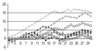
Fig. 1. Graph of Mesopotamia (diamonds), Iran (squares), Anatolia (triangles), Egypt (light x's), Palestine (dark ж's), Syria/Levant (hexagons), and the Gulf (crosses). There are two groupings apparent, Egypt, the Gulf, and Syria/Levant, and Mesopotamia, Iran, Anatolia, and Palestine. The former three show an increase in the economic status before the terminal collapse, and the latter four remain depressed from about 1700 onward.
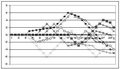
Fig. 2. Graph of the economic fluctuations of the areas adjacent to the eastern Mediterranean region represented in Fig. 1 including the Aegean/Indus (diamonds), Eastern Mediterranean (squares), Western Greece (triangles), Central Mediterranean (light x's), Central Europe (dark ж's), Asia (polygons), Steppe (hatches), and China (dark rectangles). Note that all regions exhibit a down turn toward the end of the Bronze Age.
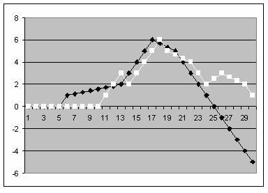
Fig. 3. Graph of the economic fluctuations of Western Greece (squares) and the Aegean/Indus (diamonds). Note the synchrony from 1000 to 2400
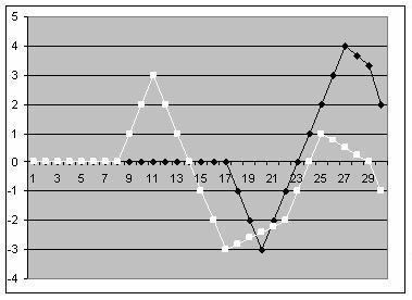
Fig. 4. Graph of the economic fluctuations of the Eastern Mediterranean and Central Europe. Note the synchrony between 700 and 2500
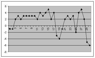
Fig. 5. This graph represents a summation of all the data per century for the regions represented in Figures 1 and 2. Note the significant troughs at 1900, 2600, and 3000 years.
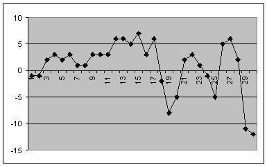
Fig. 6. This graph represents the summation of economic changes per century through the Bronze Age for the regions represented in Fig. 1. Note the troughs at 1900, 2500, and 3000 years.
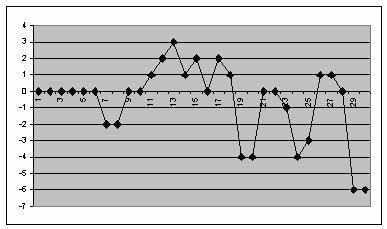
Fig. 7. This graph represents the summation of economic contractions and expansions for all the regions represented in Table 3 of Frank and Thompson (2005). The troughs at 1900, 24–2500, and 2900 are an apparent match with the form of the graphs of both Fig. 1 of this paper and a summation of Fig. 1 and Fig. 2. The trough between 600 and 900 is interesting, because it is not matched by a similar down turn in Figure 6.
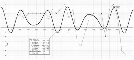
Fig. 8. This graph represents an FFT fit to the data of Fig. 6 and includes all the data for Mesopotamia, Iran, etc. The form of this graph is similar to that of Fig. 10 and clearly shows the three distinctive troughs at 1900, 2400, and 3000. These correspond to 2200 BCE, 1650 BCE, and 1300 BCE. The specific equation for the imposed curve is:
E = -2.01sin[(2π/567)(T – 604)] + .073sin[(2π/400)(T + 154)],
where E represents the relative economic status of the world system, T represents time, and the numerical constants are as given in the dialogue box in the graph.
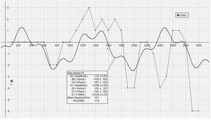
Fig. 9. The graph above represents an FFT fit of the data from Figure 7 which represents the Indus/Aegean region et al. The form of the graph is a relatively close fit to the actual data. However, the Middle Bronze Age collapse, on this graph falling between 2200 and 2600, is represented by a barely perceptible trough at approximately 2300. The specific equation for the imposed curve is:
E = -1.41sin[(sin2π/1129)(T – 541)] + .494sin[(2π/316)(T – 142/)],
where the symbols are as defined in Fig. 8.
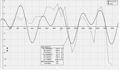
Fig. 10. The graph above represents an FFT fit of the data represented in Figure 5. Note that the events terminating the Early, Middle, and Late Bronze Ages are reasonably faithfully represented by the model. The specific equation for the imposed curve is:
E = -3.03sin[(2π/1050)(T – 621)] + 3.37sin[(2π/550)(T + 176)],
where the symbols are as in Fig. 8.