The Relationship between the Accuracy of Cultural Transmission and the Strength of Cultural Attractors

Journal: Social Evolution & History. Volume 17, Number 2 / September 2018
DOI: https://doi.org//10.30884/seh/2018.02.03
On the basis of Dan Sperber's model of cultural attraction (Sperber 1996), it is verified how various levels of cultural transmission accuracy influence the role of cultural attractors with different strengths. To this end, a simulation model is used, in which cultural representations are transmitted in a continuous space of possibilities. The conclusion is that the role of cultural attractors is enhanced (more cultural representations are going to be concentrated in the vicinity of attractors) when the cultural transmission is relatively faithful. Thereby, weak forces of attraction can be substituted by accurate transmission and the influence of strong attractors can be neutralized by too unfaithful transmission. This applies especially to cultural transmissions where large random modifications of the original cultural item are allowed rather than in case of constant error during copying.
1. INTRODUCTION
The discussion on the role of relative fidelity of cultural transmission is at the centre of the debate between two schools of evolutionary thought in cultural dynamics: the standard cultural evolution approach (originated by Cavalli-Sforza, Feldman 1981 and Boyd, Richerson 1985) and the cultural attraction theory (Sperber 1996; Cladière et al. 2014; Morin 2016). The former one treats adequate cultural transmission accuracy as the main reason for cultural stability, the latter sees cultural transmission as a process of reconstruction that involves a biased transformation in the direction of cultural attractors (Driscoll 2011).
The idea of attractors aims to explain why, in spite of inaccurate copying of cultural traits during cultural transmission, on the macro-level,
cultural traits are relatively stable within whole populations and across
generations (Cladière et al.
2014). A cultural attractor is a subset of possible
variants of a cultural trait, to which cultural traits converge during its
transmission and transformation. The convergence is the result of unequal
probability of different transformations, since the transformations in direction
of cultural attractors are more likely. It should be mentioned that the
attractor ‘is an abstract, statistical construct, like a mutation rate or
a transformation probability’ (Sperber 1996: 111–112)
and it can be a result of combining natural selection, guided-variation, psychological factors
and ecological factors (Cladière et al. 2014).
The purpose of this research is to verify, on the basis of a modified Sperber's attraction model, how various levels of inaccuracy of cultural transmission and transformation of cultural trait influence the long-term distribution of cultural traits in the space of possibilities. The problem seems important because the reconstructive and preserving character of cultural transmission is an empirical question and it could be different in different cultural domains (Acerbi and Mesoudi 2015; Driscoll 2011). For this reason, the conditions which conduce to the various patterns of cultural traits distribution deserve a thorough investigation. To achieve this goal, a simulation experiment based on the model presented by Sperber (1996: 109–112) will be carried out. The results of assumptions of different levels of infidelity and degrees of transformation during cultural transmission are going to be compared with the results of assumptions of different strengths of cultural attractors. This will enable the verification of whether greater accuracy in cultural transmission could substitute the weaker influence of attractors.
The article consists of the following sections: the description of Sperber's attraction model and the reconsideration of its limitations, detailed specification of the simulation model, report of the results and, in the last section, discussion.
2. THE ATTRACTION SIMULATION MODEL: A RECONSIDERATION
Sperber proposed an approach which describes culture as chains of cultural transmissions where cultural representations are transmitted from one individual to another by the manifestations of public representations, and are stored and processed in an individual's brain as mental representations. He called this approach ‘the epidemiology of representations’ (Sperber 1996). Since the transmission of cultural representations is never or rarely a faithful copying, during each single process of transmission the cultural trait is modified. Some modifications are more likely than others. We could imagine all possible variants of cultural traits as a set of possibilities and each cultural representation as occupying one of the possibilities. During the transmission of cultural traits, cultural representations are transforming and change their position in the set of possibilities. When some possibilities are more attractive than others (e.g., more memorisable, more interesting) – i.e. there are ‘cultural attractors’ – then transformation toward them is more probable than transformation in other directions. The distribution of the probabilities of transforming cultural traits which are positively dependent on the distance to the attractor is the effect of what is called the ‘forces of attractions’.
Sperber illustrated this phenomenon by a simple toy-model. The model assumes that there is a population of cultural items in one of 100 types. Each type is a possible state of a cultural trait, and the types can be represented in a discrete space of possibilities (the 10 × 10 grid). In each ‘generation’ every cultural item creates some descendant and dies. Sperber wanted to explain the situation when cultural traits are mostly and stably concentrated around few possibilities and not uniformly distributed over all types as they were at the start. He showed that the solution does not require the assumption of faithful replication during cultural transmission. Even if the offspring is always in a different type than its parent (because items beget into neighbour cells), thanks to not equiprobable distribution of the offspring type (positively correlated to the distance to attractors), the observed final distribution of cultural traits is concentrated around the attractors. The difference in frequencies of the types can be explained only by the differences in the probabilities of given transformations.
According to Sperber, the model has also an illustrative function, showing how cultural transmission should be modelled. However, this illustration has some limitations. The first problem concerns the interpretation of the model in the perspective of ‘epidemiology of representations’. The ontology of epidemiology of representations requires sequences of creation and production of mental and public representations. Are cultural items mental or public ones? An additional problem is that the definition of ‘cultural attractors’ seems unclear, and as Acerbi and Mesoudi (2015) noticed, in the writings of the proponents of the cultural attraction theory, an inconsistency between a dual understanding of this concept is discernible. One, which covers any directional change in cultural evolution, whether due to transformations of cultural traits during transmission or not, and second, which seems more like guided-variation (Boyd and Richerson 1985).
Secondly, in Sperber's model, many additional hidden conditions on the process of attraction are imposed. The rule that the offspring of a cultural item can adopt only one of the nearest types for the parent type interposes the assumption of some resemblance between the transformed cultural trait and the parental one. The important question is whether the degree of resemblance influences the long-termed distribution of cultural items in the model. Does more faithful transmission result in more stable distribution which is more concentrated around attractors? Additionally, the 10 × 10 grid which represents the space of possibilities assumes the discrete character of modifications of cultural traits. Therefore, it hinders the control of minor differences in the level of accuracy of cultural transmission. As it was mentioned above, we should expect that the level of fidelity of transmission should be different in various cultural domains – hence the role of these differences could be relevant for explaining real-world cultural phenomena. The continuous character of cultural representations modifications seems also more reliable (Atran 2001).
Furthermore, there
are another hidden assumptions: Sperber's toy-model is linked to his suggestion
that the multiplicity and varying number of sources of new cultural items is a
typical aspect of cultural evolution (Sperber 1996: 111). In his illustration, each cultural item had
only one descendant and only one parent. Some of the remarks concerning the cultural
attraction theory could be also applied to the model, namely that
a cultural item is the subject of attraction forces as a whole, not on the
level of its components, and that cultural attractors are stable over time and
universal for a given population (Driscoll 2011).
In this paper, the limitations of a discrete space of possibilities and lack of control of the level of fidelity of transmission are challenged. The choice to loosen up the constraints is driven by the fact, that the level of fidelity of transmission seems crucial to Sperber's explanation of the stability of culture and concentration of cultural items around attractors. Cultural attractors could work even if cultural transmission is inaccurate. But how inaccurate (as it was mentioned above, Sperber's model requires some level of fidelity)? And how strong the attractors should be?
The main hypothesis is that the inaccuracy of cultural transmission makes the attractors weaker and that stronger attractors require less accuracy. To prove this hypothesis, a simulation experiment based on the Sperber's model will be conducted.
3. SIMULATION
3.1. General objectives and assumptions of the simulation
The main objective of the simulation experiment is to answer the question of how various levels of the fidelity of cultural transmission influence the effect of attraction forces. Different degrees of transmission inaccuracy should lead to different distributions of cultural items around attractors. The simulation model is based on Sperber's attraction model (Sperber 1996: 109–112) with the following extensions:
the possibility of controlling the degree of transformation of cultural item during cultural transmission;
the continuous space of possibilities to reflect the evolution of continuous cultural traits;
the possibility of controlling the strength of attractors.
The model describes the evolution of cultural items in a space of possibilities with attractors. It assumes that cultural attractors are stable and do not change their strength and location in the long term. Also, it posits that the forces of attraction are working on the whole cultural trait rather than on its components.
3.2. Specification
Space of possibilities
The model assumes a square continuous space of possibilities of cultural items with two attractor possibilities (the attractors). One cultural item occupies only one point in the space of possibilities. In the space, the distance between two points reflects the similarity between two cultural items which are represented by these points. Two points are chosen as ‘attractors’.
The space of possibilities is limited within borders, so it is not a torus. A toroidal space would assume that border items are similar. But we should rather expect that there are some such extreme cultural traits that more extreme items are getting out of the space of possibilities and which are extremely mutually different (imagine an ideological spectrum where extreme ideologies are totally antagonistic).
Cultural items
At each step of the simulation, the cultural item begets m descendants in its neighbourhood and disappears. The position of the descendant in a space of possibilities is randomly chosen within an annulus with given inner and outer radii (respectively ri and ro), and with the centre at the point occupied by parental item. ri means the minimal dissimilarity between parental and descendant cultural item. ro means the maximal similarity between both cultural traits. ri and ro describe the fidelity of cultural transmission and the degree of transformation of the cultural trait. The longer inner radius, the less faithful is the cultural transmission. The longer outer radius, the more transformed the cultural item could be.
In
the same step, some of the descendant cultural items are selected to form a
model for cultural items, while the rest of them disappear. If cultural items are uniparental, only one descendent is chosen to be
a model. In the next step, the chosen item becomes the new cultural item which
begets new traits. The probability of the choice of a descendant to survive is
inversely proportional to the distance between the cultural item and the
nearest attractor (measured by an Euclidean distance):
 [1]
[1]
where pi is the probability of choosing a given descendant item (i) to survive from m descendants, and di is the Euclidean distance between the item i and the nearest attractor. Thanks to that mechanism, the attraction process is probabilistic (Cladière and Sperber 2007), a is the exponent which describes the strength of attractor: the greater the value of a, the stronger is the attractor.
The process of begetting new descendants and randomly choosing one of them to survive is a continuous counterpart to the item which begets a descendant of the discrete type of a neighbouring cell in the Sperber's model. But it also has an ‘epidemiological’ interpretation which is presented in the next section.
Table 1
List of the simulation model parameters
|
n |
The number of cultural items |
|
m |
The number of descendants of single cultural items in each step of simulation |
|
ri |
The inner radius of annulus area in which the type of descendant cultural item is sampling |
|
ro |
The outer radius of annulus area in which the type of descendant cultural item is sampling |
|
a |
The strength of attractors |
Simulation steps
Summing up, the steps in the simulation process are as follows:
1. Cultural items are placed randomly in the continuous space of possibilities.
2. At each next step, each cultural item:
2.1. begets m descendants in a random location within an annulus with the centre at the position of cultural item (the inner radius of the annulus is equal to ri, and outer radius is equal to ro);
2.2. one of the descendants is selected to survive in the next step, the rest of them die. The distribution of the probability of survival is determined by the distance between the descendant position and the position of the nearest attractor, according to Equation [1].
3.3. Interpretation
One of the problems with Sperber's description of his model was the lack of an epidemiological interpretation, which requires a chain of mental representations triggering public representations triggering other mental representations, and so on. It is not clear whether the cultural items are public or mental representations, and what the link between begetting descendants by parental item and cultural transmission is. We only can read it as a process of copying cultural traits from one agent to another. The choice of a descendant type among neighbours means that copied traits are not identical to parental traits (Sperber 1996: 111).
If we assume that cultural items are mental representations, in the model presented above, the begetting of descendants of culture items can be interpreted as creating various public representations (for example retellings of the same story). The selection of the descendant to survive is a counterpart of the process of memorizing the most attractive version which is stored as a mental representation. The rest of the descendants disappear, as less attractive versions are forgotten.
If cultural items are equated with public representations, then the begetting of descendants is a counterpart of the process of recognising the public representations by people who are storing the inaccuracy memories about them. The selection of the descendant to survive can be interpreted as the phenomenon where the most lasting and the most attractive memories trigger the production of public representations.
In the first case, the parameter m is proportional to the frequency of manifestations of a cultural representation. In the latter, m reflects the number of viewers/listeners.
4. EXPERIMENTS AND RESULTS
4.1. Experiment design
The model is implemented within Mesa: the agent-based modelling framework in Python 3+. Six simulations are conducted: each one using different parameter settings. Three scenarios assume three different strengths of attractors (a = 1, a = 0.5 and a = 2). In each scenario, three cases of inaccuracy of cultural transmission will be verified. The first, when the minimal possible transmission error is low (ri is near 0) and the degree of transformation is low (ro < 1); the second, when the minimal possible transmission error is high (ri > 1) and the degree of transformation is high (ro > 2); and the third one when the minimal possible transmission error is low and the degree of transformation is high (ri is near 0, ro > 2).
Since no interactions between agents occur, a sufficiently large number of cultural items should give representative results. The robustness of the results will be checked based on the different place of attractors (robustness with regard to the location of attractors) and with regard to the number of descendants of a single cultural item (robustness with regard to parameter m). The default parameter settings are listed in the following table (Table 2).
Table 2
Default simulation parameter settings
|
Parameter |
Default value |
|
n |
1000 |
|
ri, ro |
1. ri = 0.01, ro = 0.75 (low transmission error and low degree of transformation) 2. ri = 1.25, ro = 2.25 (high transmission error and high degree of transformation) 2. ri = 0.01, ro = 2.25 (low transmission error and high degree of transformation) |
|
m |
5 |
|
minimal and maximal coordinates of space |
minimal x: 0; maximal x: 10 minimal y: 0; maximal y: 10 |
|
attractor positions (x,y) |
North-East: (6.5, 7.5), South-West: (3.5, 2.5) |
|
a |
1. a = 1 2. a = 0.5 3. a = 2 |
4.2. Results
Scenario I: a = 1
The first test examines the distribution of cultural items when the strength of attractors is a = 1. The distributions of cultural items after 1000 iterations for three cases of error and transformation parameters are presented in Figures 1a – 1b (the continuous space was reprojected onto the 10 × 10 grid). The snapshots of the last (1000th) iteration (Fig. 1a) show whether the model converges to the state of concentration of cultural items around attractors. The distributions of items cumulated over all iterations (Fig. 1b) show the stability of the concentration of cultural items around the attractors.
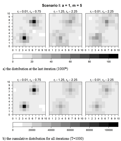
Fig. 1. Distribution of cultural items at the final
iteration
and cumulative (a = 1)
Source: Author's calculations.
The plots indicate that the distribution that is most concentrated around attractors is obtained in the case of relatively low transmission errors and small transformations (small ri and ro). A more dispersed distribution is obtained with higher values of ri and ro. In the last iteration, 39 per cent of cultural items are placed within a distance of 1 from one of the attractors when the transmission error is low and the degree of transformation is low. When the faithfulness is weaker, the attractors group 17 per cent (ri = 1.25, ro = 2.25) or 20 per cent (ri = 0.01, ro = 2.25) of cultural items. Due to the potential influence of boundaries of the cultural space (existence of the corners and the edges) it should be mentioned that also the relative concentration around attractors (the ratio of the percentage of cultural items within a distance of 1 from to attractors to the percentage of cultural items within a distance of 2) is the highest for the most faithful case. The detailed results are presented in Table 3.
Table 3
Results of simulations (a = 1)
|
|
Median concentration around attractors d = 1 |
Median concentration around attractors d = 2 |
MAD of the ratios of concentrations around both attractors d = 1 |
MAD of the ratios of concentrations around both attractors d = 2 |
Ratio of concentration within d = 1 to concentration
within |
|
ri = 0.01; ro = 0.75 |
0.393 |
0.661 |
0.071 |
0.047 |
0.595 |
|
ri = 1.25; ro = 2.25 |
0.172 |
0.461 |
0.127 |
0.076 |
0.375 |
|
ri = 0.01; ro = 2.25 |
0.208 |
0.499 |
0.108 |
0.070 |
0.418 |
Source: Author's calculations. Concentration – the amount of cultural items within a distance of d divided by the total number of items; ratio of concentrations around both attractors – the concentration around the North-East attractor divided by the concentration around the South-West attractor; median concentration – the median of the 1000 iterations; MAD – mean absolute deviation.
A visible difference between the case of high transmission error and high degree of transformation, and the case of low transmission error and high degree of transformation is noticeable. The former is characterised by lower concentration around the attractors, lower relative concentration around the attractors, but also by stronger fluctuations of the ratios of concentrations around the North-East attractor to the concentrations around the South-West attractor (manifested by greater mean absolute deviation of the ratios, see Fig. 2b). The last characteristic means that a higher transmission error makes the cultural attractors less stable.
It is important to notice that the above-described results are representative for the sample of 200 simulation runs (each conducted for three parameter settings – the results are shown in Table 6a). Moreover, the distribution of cultural items is stable and after 100 iterations no major changes in the concentration of cultural items are observed (Fig. 2).
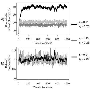
|
a) Concentration of cultural items within a distance of 1 from attractors |
|
b) The ratios of concentrations around both
attractors (i.e. the concentrations around the NE attractor divided by the
concentrations around the SW attractor), |
Fig. 2. Evolution of the distribution of cultural items in simulations
Source: Author's calculations.
Scenario II: a = 0.5
The same experiment
was conducted with different settings where the attractors' strength was weaker
(a = 0.5). The weaker forces of attraction
should make the distribution of cultural items less concentrated around
attractors. As shown in the snapshots from simulations (of the last iterations – Fig. 3a) and in the plots of cumulative
distribution over all iterations
(Fig. 3b), the cultural items are more dispersed than in the case of
a = 1. The distribution which is most
concentrated around the attractors is obtained in the case of low transmission
error and low degree of transformation. The most dispersed distribution occurs
in the case of high error and high degree of transformation. The observation is
confirmed by the detailed results presented in Table 4. As it can be compared
with the results of 200 simulation runs for each of the three parameter
settings (Table 6b), the above results are representative.
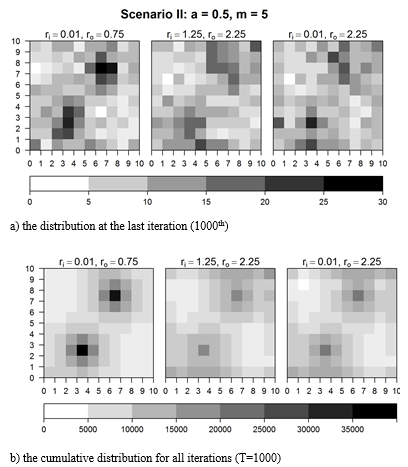
Fig. 3. Distribution of cultural items at the final iteration and cumulative (a = 0.5)
Source: Author's calculations.
Table 4
Results of simulations (a = 0.5)
|
|
Median concentration around attractors d = 1 |
Median concentration around attractors d = 2 |
MAD of the ratios of concentrations around both attractors d = 1 |
MAD of the ratios of concentrations around both attractors d = 2 |
Ratio of concentration
within |
|
ri = 0.01; |
0.170 |
0.421 |
0.114 |
0.056 |
0.404 |
|
ri = 1.25; |
0.103 |
0.320 |
0.162 |
0.089 |
0.321 |
|
ri = 0.01; |
0.114 |
0.337 |
0.149 |
0.085 |
0.338 |
Source: Author's calculations. Concentration – the amount of cultural items within a distance of d divided by the total number of items; ratio of concentrations around both attractors – the concentration around the North-East attractor divided by the concentration around the South-West attractor; median concentration – the median of the 1000 iterations; MAD – mean absolute deviation.
The percentages of cultural items which are near the attractors (within a distance of 1, within a distance of 2 and relative amount of cultural items within a distance of 1 and 2) are lower than in the case of stronger attraction forces. It can be noticed that the results for the case of a = 1, ri = 1.25, ro = 2.25 (the higher transmission error and highest transformation) and for the case of a = 0.5, ri = 0.01, ro = 0.75 are similar. This indicates that the fidelity of transmission can substitute for the weakening of the attraction forces.
Scenario III: a = 2
In the last scenario, the influence of an increase in the attractors' strength was checked. The plots (Figs 4a – 4b) and data in Table 5 show that the distributions of cultural items are more concentrated around attractors than in the previous scenarios. As in the former simulations results, the least dispersed distribution is obtained in the case of low transmission error and low degree of transformation and the most dispersed one occurs in the case of high error and high degree of transformation.
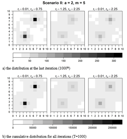
Fig. 4. Distribution of cultural items at the final iteration and cumulative (a = 2)
Source: Author's calculations.
The differences between the concentrations around attractors among the three types of transmission are larger than in the scenarios of weaker attractors. In the most faithful case, the concentration within a distance of 1 is over 82 per cent, which leads to a high relative concentration of cultural items within a distance of 1 to the concentration within a distance of 2. Stronger attraction forces bolster the influence of a high fidelity transmission on the cultural items grouping around the attractors.
Table 5
Results of simulations (a = 2)
|
|
Median concentration around attractors d = 1 |
Median concentration around attractors d = 2 |
MAD of the ratios of concentrations around both attractors d = 1 |
MAD of the ratios of concentrations around both attractors d = 2 |
Ratio of concentration within |
|
ri = 0.01; |
0.821 |
0.949 |
0.030 |
0.019 |
0.864 |
|
ri = 1.25; |
0.289 |
0.673 |
0.092 |
0.058 |
0.430 |
|
ri = 0.01; |
0.388 |
0.745 |
0.079 |
0.055 |
0.522 |
Source: Author's calculations. Concentration – the amount of cultural items within a distance of d divided by the total number of items; ratio of concentrations around both attractors - the concentration around the North-East attractor divided by the concentration around the South-West attractor; median concentration – the median of the 1000 iterations; MAD – mean absolute deviation.
It can be noticed
that the results from the case of the highest transmission error and the
highest degree of transformation (a =
2, ri = 1.25, ro = 2.25) under the
strengthened forces of attraction are similar to the results from the case of
the lowest transmission error and the lowest degree of transformation (a = 1, ri = 0.01, ro
= 0.75). It means that stronger attraction forces can substitute low
faithfulness of the cultural trans-
mission.
Robustness
As mentioned above, the illustrative results are representative for the sample of results obtained over 200 simulation runs, which were computed for each scenario. The summary of the results is shown in Table 6.
Table 6
Median, first and ninth decile of the distributions of the statistical results obtained over 200 runs and at the last iteration
a) Parameter setting: m = 5, a = 1
|
|
ri = 0.01; ro = 0.75 |
ri = 1.25; ro = 2.25 |
ri = 0.01; ro = 2.25 |
||||||
|
med |
1. dec |
9. dec |
med |
1. dec |
9. dec |
med |
1. dec |
9. dec |
|
|
Concentration around attractors, d = 1 |
0.391 |
0.388 |
0.395 |
0.173 |
0.172 |
0.173 |
0.208 |
0.208 |
0.209 |
|
Concentration around attractors, d = 2 |
0.659 |
0.655 |
0.664 |
0.461 |
0.460 |
0.463 |
0.500 |
0.499 |
0.502 |
|
MAD of the ra- |
0.073 |
0.061 |
0.088 |
0.123 |
0.118 |
0.128 |
0.111 |
0.105 |
0.117 |
|
MAD of the ra- |
0.051 |
0.040 |
0.067 |
0.074 |
0.069 |
0.080 |
0.070 |
0.064 |
0.078 |
|
Ratio of concentration within d = 1 to concentration within d = 2 |
0.594 |
0.591 |
0.596 |
0.374 |
0.373 |
0.375 |
0.417 |
0.416 |
0.418 |
b) Parameter settings: m = 5, a = 0.5
|
|
ri = 0.01; ro = 0.75 |
ri = 1.25; ro = 2.25 |
ri = 0.01; ro = 2.25 |
||||||
|
med |
1. dec |
9. dec |
med |
1. dec |
9. dec |
med |
1. dec |
9. dec |
|
|
Concentration around attractors, d = 1 |
0.169 |
0.166 |
0.172 |
0.103 |
0.103 |
0.104 |
0.114 |
0.114 |
0.115 |
|
Concentration around attractors, d = 2 |
0.417 |
0.412 |
0.422 |
0.321 |
0.320 |
0.322 |
0.338 |
0.337 |
0.340 |
|
MAD of the ra- |
0.119 |
0.108 |
0.135 |
0.161 |
0.155 |
0.167 |
0.152 |
0.145 |
0.160 |
|
MAD of the ra- |
0.071 |
0.059 |
0.089 |
0.089 |
0.084 |
0.094 |
0.086 |
0.081 |
0.093 |
|
|
ri = 0.01; ro = 0.75 |
ri = 1.25; ro = 2.25 |
ri = 0.01; ro = 2.25 |
||||||
|
med |
1. dec |
9. dec |
med |
1. dec |
9. dec |
med |
1. dec |
9. dec |
|
|
Ratio of concentration
within |
0.405 |
0.402 |
0.408 |
0.322 |
0.321 |
0.323 |
0.338 |
0.337 |
0.339 |
c) Parameter settings: m = 5, a = 2
|
|
ri = 0.01; ro = 0.75 |
ri = 1.25; ro = 2.25 |
ri = 0.01; ro = 2.25 |
||||||
|
|
med |
1. dec |
9. dec |
med |
1. dec |
9. dec |
med |
1. dec |
9. dec |
|
Median concentration around attractors, d = 1 |
0.818 |
0.816 |
0.820 |
0.289 |
0.288 |
0.289 |
0.388 |
0.387 |
0.389 |
|
Median concentration around attractors, d = 2 |
0.948 |
0.946 |
0.950 |
0.672 |
0.671 |
0.673 |
0.745 |
0.744 |
0.746 |
|
MAD of the ra- |
0.031 |
0.026 |
0.040 |
0.094 |
0.089 |
0.100 |
0.080 |
0.073 |
0.087 |
|
MAD of the ra- |
0.021 |
0.016 |
0.034 |
0.060 |
0.054 |
0.068 |
0.055 |
0.048 |
0.065 |
|
Ratio of concentration within d = 1 |
0.863 |
0.861 |
0.864 |
0.430 |
0.429 |
0.431 |
0.521 |
0.520 |
0.522 |
Source: Author's calculations. Concentration - the amount of cultural items within a distance of d divided by the total number of items; ratio of concentrations around both attractors – the concentration around the North-East attractor divided by the concentration around the South-West attractor; median concentration – the median of the 1000 iterations; MAD – mean absolute deviation.
The results confirm a robust relationship between the fidelity of transmission and the distribution of cultural items. Low-error and weak transformative transmission furthers a stronger concentration of cultural items around attractors, while in the opposite case the role of attractors becomes less relevant. The biggest difference between various types of transmission is noticeable between the most and the least transformative one (i.e. with regard to the parameter ro). Increasing possibilities of random transformations of a cultural trait are disturbing an attractor-concentrated distribution more than an every-time error in copying.
The robustness of the results with regard to the number of single cultural item's descendants (m) and the location of attractors was also checked. Scores are presented in Table A.1 (in the Appendix). For each alternative set of the parameters, the positive relationship between the fidelity of transmission and the concentration of cultural items around attractors was confirmed. However, there was a problem with a small number of single cultural item's descendants (the case of m = 2), because many items were concentrated in corners of the cultural space. This simulation artefact was more explicit when the transmission was more transformative and high-error. But that can be interpreted just as the result of weakening of the attractors.
5. DISCUSSION
The main contribution of the paper is the demonstration that the fidelity of transmission could substitute the forces of attraction and vice versa. Weak forces of attraction can be enhanced by accurate transmission and the influence of strong attractors can be neutralized by excessively unfaithful transmission. This applies especially to cultural transmissions in which large modifications of the original cultural item are allowed. The every-time error in copying seems to be less relevant.
This has serious theoretical and empirical implications. While the debate between dual inheritance theorists and cognitive anthropologists is mainly focused on the defence of accuracy or attraction forces in creating stability in the transmission of cultural traits, the simulation shows that they are both important for explaining this problem and next question should be formulated ‘how much accuracy is necessary to stabilize the transmission of cultural traits with a given strength of attraction forces’. Answering this question requires empirical studies. However, many cultural phenomena are reflected only in the data showing the distribution of cultural items (such as archaeological data of material culture). If accuracy can substitute attraction forces, and it leads to the same effect of concentration, how can one distinguish between these two cases?
The other implications of above research concern the problem of cultural diversity. If attraction forces are relatively weak and large modifications of transmitted cultural items are allowable, then the distribution of cultural items in cultural space is quite dispersed. Thus, the cultural diversity is sustained even after long periods of attractors influence.
The presented model can be extended in various
directions. The simulation specification could be made more realistic – for example by assuming the multiparental cultural items (Sperber 1996: 111), or by the calibration of the parameters to real
cultural phenomena. The succeeding models could focus more on exploiting the
interpretation within the ‘epidemiology of representation’ framework, i.e. use some additional assumptions
about the difference between mental and public representations. The model is
also
a potential basis for a research of more complex
cultural processes – for example the influence of density of cultural representations in
the vicinity of attractors on the strength of the attractors (as Sperber
suggests: an increase in the density of public representations around the
attractor should reinforce it, and an increase in the density of mental
representations should decrease its relevance and weaken the attractor – 1996: 115–116).
REFERENCES
Acerbi, A., and Mesoudi A. 2015. If We Are All Cultural Darwinians What's the Fuss about? Clarifying Recent Disagreements in the Field of Cultural Evolution. Biology & Philosophy 30 (4): 481–503.
Atran, S. 2001. The Trouble with Memes. Inference versus Imitation in Cultural Creation. Human Nature 12 (4): 351–381.
Boyd, R., and Richerson, P. J. 1985. Culture and the Evolutionary Process. Chicago: Chicago University Press.
Cavalli-Sforza, L. L., and Feldman, M. 1981. Cultural Transmission and Evolution: A Quantitative Approach. Princeton: Princeton University Press.
Cladière, N., and Sperber, S. 2007. The Role of Attraction in Cultural Evolution. Journal of Cognition and Culture 7 (1–2): 89–111.
Cladière, N., Scott-Phillips, T. C., and Sperber, D. 2014. How Darwinian is Cultural Evolution? Philosophical Transactions of Royal Society 369 (1642): 20130368.
Driscoll, C. 2011. Fatal Attraction? Why Sperber's Attractors do not Prevent Cumulative Cultural Evolution. British Journal for the Philosophy of Science 62 (2): 301–322.
Morin, O. 2016. Reasons to be Fussy about Cultural Evolution. Biology & Philosophy 31(3): 447–458.
Sperber, D. 1996. Explaining Culture. The Naturalistic Approach. Oxford: Blackwell Publishing.
Appendix
Table A.1
Median, first and ninth decile of the distributions
of the statistical results obtained
over 200 runs and
at the last iteration – alternative
parameter settings
a) Parameter setting: m = 2, a = 1
|
|
ri = 0.01; ro = 0.75 |
ri = 1.25; ro = 2.25 |
ri = 0.01; ro = 2.25 |
||||||
|
med |
1. dec |
9. dec |
med |
1. dec |
9. dec |
med |
1. dec |
9. dec |
|
|
Median concentration around attractors, d = 1 |
0.197 |
0.194 |
0.199 |
0.104 |
0.104 |
0.105 |
0.116 |
0.116 |
0.117 |
|
Median concentration around attractors, d = 2 |
0.461 |
0.457 |
0.466 |
0.332 |
0.331 |
0.334 |
0.353 |
0.351 |
0.354 |
|
MAD of the ratios of concentrations around both
attractors, |
0.108 |
0.096 |
0.125 |
0.160 |
0.153 |
0.166 |
0.151 |
0.144 |
0.157 |
|
MAD of the ratios of concentrations around both
attractors, |
0.063 |
0.055 |
0.083 |
0.087 |
0.082 |
0.093 |
0.084 |
0.078 |
0.091 |
|
Ratio of concentration within d = 1 to concentration within d = 2 |
0.426 |
0.424 |
0.429 |
0.314 |
0.312 |
0.315 |
0.330 |
0.329 |
0.331 |
b) Parameter setting: m = 9, a = 1
|
|
ri = 0.01; ro = 0.75 |
ri = 1.25; ro = 2.25 |
ri = 0.01; ro = 2.25 |
||||||
|
med |
1. dec |
9. dec |
med |
1. dec |
9. dec |
med |
1. dec |
9. dec |
|
|
Median concentration around attractors, d = 1 |
0.472 |
0.469 |
0.476 |
0.203 |
0.202 |
0.204 |
0.253 |
0.252 |
0.254 |
|
Median concentration around attractors, d = 2 |
0.722 |
0.718 |
0.728 |
0.509 |
0.508 |
0.511 |
0.556 |
0.555 |
0.558 |
|
MAD of the ratios of concentrations around both
attractors, |
0.062 |
0.054 |
0.074 |
0.113 |
0.108 |
0.119 |
0.101 |
0.095 |
0.107 |
|
MAD of the ratios of concentrations around both
attractors, |
0.044 |
0.035 |
0.059 |
0.070 |
0.065 |
0.076 |
0.066 |
0.061 |
0.074 |
|
Ratio of concentration within d = 1 to concentration
within |
0.654 |
0.651 |
0.656 |
0.399 |
0.398 |
0.400 |
0.455 |
0.454 |
0.456 |
c) Parameter setting: different localisations of two attractors, m = 5, a = 1
|
|
ri = 0.01; ro = 0.75 |
ri = 1.25; ro = 2.25 |
ri = 0.01; ro = 2.25 |
||||||
|
med |
1. dec |
9. dec |
med |
1. dec |
9. dec |
med |
1. dec |
9. dec |
|
|
Median concentration around attractors, d = 1 |
0.426 |
0.400 |
0.481 |
0.220 |
0.177 |
0.302 |
0.257 |
0.214 |
0.335 |
|
Median concentration around attractors, d = 2 |
0.674 |
0.651 |
0.702 |
0.528 |
0.489 |
0.602 |
0.559 |
0.523 |
0.624 |
|
MAD of the
ratios of concentrations around both attractors, |
0.090 |
0.061 |
0.155 |
0.120 |
0.078 |
0.162 |
0.109 |
0.076 |
0.140 |
|
MAD of the
ratios of concentrations around both attractors, |
0.064 |
0.036 |
0.150 |
0.070 |
0.041 |
0.085 |
0.069 |
0.039 |
0.087 |
|
|
ri = 0.01; ro = 0.75 |
ri = 1.25; ro = 2.25 |
ri = 0.01; ro = 2.25 |
||||||
|
|
med |
1. dec |
9. dec |
med |
1. dec |
9. dec |
med |
1. dec |
9. dec |
|
Ratio of concentration within d = 1 to concentration within d = 2 |
0.634 |
0.595 |
0.709 |
0.416 |
0.350 |
0.550 |
0.460 |
0.397 |
0.585 |
Source: Author's calculations. Concentration – the amount of cultural items within a distance of d divided by the total number of items; ratio of concentrations around both attractors - the concentration around the one of the attractors divided by the concentration around the second attractor; median concentration – the median of the 1000 iterations; MAD – mean absolute deviation; med – median; 1. dec – first decile; 9.dec – ninth decile.