Measuring Globalization: Network Approach to Countries' Global Connectivity Rates and Their Evolution in Time

Authors: Shulgin, Sergey G. ; Zinkina, Julia; Andreev, Alexey I.
Journal: Social Evolution & History. Volume 18, Number 1 / March 2019

DOI: https://doi.org/10.30884/seh/2019.01.07

Traditional approaches to measuring countries' levels of globalization mostly rely on index compilation. This paper presents a new method of estimating the countries' global connectivity rates based on the degree of their involvement into the global networks of transborder flows and relations. We apply the concept of k-core from network analysis to estimate the level of countries' involvement into global networks. Changes in the countries' structural positions within these networks affect their overall connectivity rankings. In our analysis we take into account four types of networks, such as trade in goods, trade in services, foreign direct investment, and migration. However, the method easily allows for adding other networks (when sufficient data is available).

INTRODUCTION

Recent decades have seen a surge of scholarly interest in globalization – and, accordingly, a number of attempts at quantitative representation of the phenomenon. The majority of these attempts use the same format of developing globalization indices, either simple (usually these ones are related to measuring economic openness) or compound. The most widely known compound globalization indices include KOF Globalization Index (Dreher 2006), Maastricht Globalization World (Martens and Zywietz 2006; Martens and Raza 2008), A. T. Kearney/ Foreign Policy Magazine Globalization Index (A. T. Kearney Inc, Global Policy Group and Foreign Policy Magazine 2001), Global Index by TransEurope Research Network (Raab et al. 2008), New Globalization Index (Vujakovic 2010), Ernst & Young's Annual Globalization Index (Ernst and Young 2012), etc.

However, elsewhere we have shown that most globalization indices share a number of methodological drawbacks, the most significant of which consists in the indices' inability of accounting for globalization as, first and foremost, a world-scale phenomenon. Globalization rankings are calculated for individual countries on the basis of country-level values of certain indicators, but without any attention to the position of a given country in the global space of flows, networks, and relations (for the analysis of other methodological limitations of indices see Zinkina, Korotayev, and Andreev 2013).

In this paper we try to develop an essentially different approach to measuring globalization. The essence of this approach is based on the definition of globalization proposed by a prominent global politics and economics scholar George Modelski. His idea was to combine two approaches: the ‘connectivist’ approach, viewing globalization as increasing transborder interactions, relations, and flows, and the institutional approach, which explains globalization as the emergence and evolution of global, planetary-scale institutions. Let us emphasize that ‘institutions’ is a very wide term for Modelski, so this notion includes, for example, global free trade, multinational enterprises, global governance, worldwide social movements, ideologies, etc. (Modelski 2008).

We select a number of global institutions with network structure formed by transborder interactions and flows and proceed to building network models and applying network analysis methods in order to characterize the structural position of each country within these networks. We then calculate countries' global connectivity rankings based on their structural positions, and trace changes in these rankings which took place over the recent decade and a half.

DATA

When considering countries from the point of view of global networks, two major approaches can be applied. The first approach puts emphasis on the closeness of countries, including the geographical closeness (smallest distance between countries, sharing a common border, etc.), regional closeness (belonging to the same region), historical and cultural closeness (being parts of a single state in the past, sharing a common language and/or a common religion, etc.). The second approach, on which we rely in this paper, investigates the intensity of relations between countries rather than their relative proximity. We analyze four networks formed by transborder flows and relations:

· trade in goods: to calculate the values of this indicator for pairs of countries we use data on inter-country trade presented in the UN COMTRADE database according to the Harmonized Commodity Description and Coding Systems classification. Basically, we use data on the total value of import from country A to B and from B to A (in current dollar prices). In the cases of missing data on import from A to B we use data on export from B to A instead (the so-called ‘mirroring’). We are aware of the fact that this procedure can bring in certain errors, since the export statistics can differ from import statistics, but we still use it, as inexact data is still better for network models than missing data (as the latter can nullify existing connections between countries and thus distort the structure of the network);

· trade in services: data for this indicator is obtained from ‘The Trade in Services’ database which accumulates data on trade in services compiled by OECD, Eurostat, United Nations, and IMF;

· accumulated stock of bilateral FDI: data for this indicator is obtained from the United Nations COMTRADE database;

· accumulated stock of migrants: data for this indicator is obtained from the United Nations which publishes data on the migrant stocks classified by the country of origin for 197 countries of the world every five years since 1990.

When analyzing the structural changes of these networks and positions of particular countries therein over time, we divide all the available data into three consecutive time periods: 2000–2004, 2005–2009, and 2010 – current time. We lack earlier data on FDI, so for the time being we do not extend our analysis into deeper history.

NETWORK MODEL

For each of the four networks listed above we build a network model of inter-country relations based on an undirected graph. Each country is represented by a vertex in the graph. Two vertices are connected with an edge if the intensity of relation between the two countries corresponding to these vertices exceeds a certain threshold. The global connectivity rate of a given country depends on the network properties of its position in each of the four network models.

For each of the four networks we build three matrices NxN (one matrix for each of the three consecutive time periods), where N is the total number of countries, and column i presents the data on the relations of country i with all the other countries in the given network. The NxN matrix is symmetrical because the relation between countries i and j is presented as the total sum of the bilateral flow of good/services, or the total sum of the bilateral stock of migrants from i to j and from j to i. For FDI we do not use summing, but rather take the larger of the two values (FDI from i to j or from j to i).

Setting thresholds is the key question for building network models. In fact, the total number of edges (relations taken into account in the model) directly depends on the minimal value of the relation intensity (trade volume, FDI stock, or stock of migrants) set in this model. If the threshold is zero, the model will account for all the existing transborder interactions. However, zero thresholds are not particularly suitable for our purpose, as they would let into the model all transborder relations with values varying by several orders of magnitude (bilateral trade volume ranging from thousands to trillions of dollars, migration stocks varying from dozens to millions of people). Thus, in this paper we use a multitude of non-zero thresholds for each of the four networks (see ‘Network analysis’ section for more details).

A symmetrical matrix of relations can be viewed as an undirected graph, so our further investigation is based on the methods of network analysis of graphs. Our aim is to elaboarate a measure for each country which would reflect the level of its integration with all other countries.

The most basic network measure capturing the level of a vertex integration with other vertices is vertex degree, which is simply the total number of relations (edges) the given vertex has with other vertices in this graph. However, this simple measure is not perfect for the purpose of our research as the number of relations (edges) per se tells us very little about the structural position of a country within the global network. Here comes a question: Is it mostly connected to very well-connected countries, or rather to low-connected ones, or both?

That is why we apply more complex methods of network analysis related to establishing the most densely connected communities of countries within the network. There are various algorithms of network clusterization which allow to specify such communities on the graph (for reviews of such algorithms see, e.g., Anderberg 1973; Spath 1980; Fortunato 2010).

A community with the maximum possible density of interconnections is called a clique. In a clique, all elements are connected to each other. The number of vertices in the largest clique within the graph is called ‘clique number’. Ever since the notion of clique made its appearance (Luce and Perry 1949), numerous ideas and approaches to using it in graph analysis have been proposed. However, the clique approach has some limitations hindering its application to our research objective. Indeed, cliques set up a strict restriction on the number of countries (vertices) entering them, as this number is directly defined by the notion of full connectivity. In other words, in a clique consisting of 20 vertices each vertex must have 19 edges connecting it to all members of the clique. Vertices that are not fully connected to the members of the clique cannot enter it, even if they have the same (or even higher) number of edges.

Our task is to select not necessarily a completely interconnected group, but rather a group of the largest possible size with the largest possible degree of interconnectedness. For this, let us use the concept of a k-core. A k-core is a subset of vertices each of which has not less than k relations with other vertices in this subset (the idea of such subset was proposed in Seidman 1983). For a fully interconnected graph with N vertices, k = N – 1, in which case a k-core is equal to a clique. In other cases, however, k-cores tend to encompass a wider subset of vertices (which in our networks means a larger number of countries). For example, a clique with density 20 includes strictly 21 vertices, each of which has strictly 20 connections (edges) to other members of the clique. A k-core of the same density can include many more vertices (say, 40), each of which has not less than, say, 20 connections to other vertices in the k-core. The number of countries entering the k-core depends on the structure of the graph rather than on the notion of full connectedness.

Apart from reflecting the structure of the graph, the k-core metric has one more noteworthy feature. It allows us not just to find the vertices with the highest number of connections (a simple vertex degree metrics would suffice for that), but rather reveals the vertices with the greatest number of connections to other highly-connected vertices (sort of a ‘high connectivity club’).

NETWORK ANALYSIS

First, for each country (represented by a vertex) we evaluate its network characteristics in each of the four networks. The most important of these characteristics is the maximum degree of the k-core to which it belongs (we denote it as Ki). Second, we define the maximum k-core degree in the whole network, i.e., the subset with the largest possible number of connections (we denote it as Kmax). Third, we divide Ki by Kmax. The value of Ki/Kmax for a given country i equals to 1 if this country belongs to the k-core of maximum density. Otherwise, for example, Ki/Kmax = 0.5 if country i belongs to a k-core with a degree twice smaller than the maximum k-core degree in the graph. To set another example, Ki/Kmax = 0 if country i is represented by a fully isolated vertex and has no relations whatsoever with any other country (vertex) within the given network.

Thus, Ki/Kmax can attain values ranging from 0 (fully isolated country/vertex) to 1 (country/vertex belonging to the k-core with the maximum possible density of relations within the network).

EVALUATION OF GLOBAL NETWORKS WITH THE USE OF K-CORES

The method of k-core selection accounts for the number of relations (edges) between countries (vertices), but does not have any internal procedure of accounting for the intensity of relations (the weight of edges). So, the number of relations (edges) which constitute the network rather depends on the external choice of threshold levels. Higher thresholds allow for a smaller number of more intense relations (edges with greater weight) – and, vice versa, lower thresholds increase the connectivity of the network but account for less significant relations as well (i.e., the ones reflecting only rather weak integration of countries).

For each of the four networks, we use different threshold values to construct a multitude of network models with varying density. Then we proceed to evaluate the network characteristic Ki/Kmax for each vertex in each of these network models. Notably, k-cores are applicable to the analysis of networks with a rather small number of (very intense) relations. For each of the four networks we estimated 1,000 network models obtained with 1,000 thresholds chosen randomly from an even distribution U(Xmin, Xmax), where Xmin is minimum edge weight (value level) and Xmax threshold with only 5 per cent of all edges weight above that level (Xmax higher than 95 per cent of existing edge weights).

Depending on the threshold chosen, we obtain various network models with varying size and composition of k-cores. Averaging results for different thresholds, we estimate metric for each network (trade in goods, trade in serviced, FDI stocks, and migrant stocks). Results of synthesis of all four networks are presented in Fig. 1 for the most recent period; see Table 1 and Appendix 1 for the the exact values of various countries' global connectedness indices for all networks and all three consecutive periods.

The analysis of a multitude of network models with varying thresholds for the most recent period reveals that only two countries, United Kingdom and the USA, retain maximum density of relations (i.e., are connected with the maximum possible number of countries) at all threshold levels in all four dimensions. Their global connectedness level is 4 (i.e., their Ki/Kmax is 1 in each of the four networks).

The analysis of various threshold levels allows for a statistical inference of the obtained results. Analyzing the distributions obtained at various threshold levels, we can estimate confidence intervals for the resultant index. Along with United Kingdom and the USA, four more countries (Germany, France, Italy, and Spain) have maximum global connectedness level (4) in 95 per cent of all our results – in other words, they almost always belong to the group of the most interconnected countries. They are marked with black on Fig. 1.

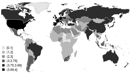
Fig. 1. Rates of Countries' Global Connectedness for the Most Recent Period (2010–current time)

‘The leaders’ are followed by a group of 19 countries including the Netherlands, Switzerland, Belgium, China, Japan, Canada, the Russian Federation, Ireland, Sweden, Australia, Poland, South Korea, Austria, Denmark, India, Brazil, Singapore, Norway, and Hong Kong (from here on countries are listed in the descending order of their global connectivity rates). These countries (marked with dark grey in Fig. 1) have global connectivity rates ranging from 3.75 to 3.99 and confidence intervals ranging from 3 to 4, which means that at certain threshold levels these countries rather regularly find themselves among the most connected ones.

Next comes a group of 23 countries with global connectivity rates ranging from 3 to 3.75, which can occasionally belong to the most connected group. These countries include Turkey, Hungary, Finland, Portugal, Czech Republic, Luxembourg, Greece, South Africa, Thailand, Malaysia, Romania, Chile, Israel, Mexico, Bulgaria, New Zealand, Slovakia, Indonesia, Cyprus, Ukraine, Philippines, Argentina, and Croatia.

As for the countries with relatively lower levels of global connectivity rates (values ranging from 2 to 3), these include Pakistan, Egypt, Lithuania, Slovenia, Latvia, Estonia, Morocco, United Arab Emirates, Malta, Venezuela, Nigeria, Iran, Saudi Arabia, Kazakhstan, Colombia, Belarus, Iceland, Vietnam, Peru, Uruguay, Kuwait, Panama, Serbia, Bangladesh, Qatar, Mauritius, Azerbaijan, Algeria, Lebanon, and Jordan. These countries are excluded from the most connected group at any threshold levels.

The rest of the countries have low (from 1 to 2) or extremely low (less than 1) rates of global connectivity.¹

THE EVOLUTION OF GLOBAL CONNECTIVITY RATES

Having calculated the global connectivity rates of various countries for three consecutive time periods (2000–2004, 2005–2009, 2010–current time) we can proceed to investigate the changes that occurred to the rates during these time periods. The largest increase in the relative position in global connectivity rankings was observed for the BRIC countries, as well as for Poland, Romania, and Chile. On the contrary, relative position in global connectivity decreased in Scandinavian countries (Sweden, Norway, and Finland), as well as in Denmark, Portugal, Hong Kong, Greece, Israel, and New Zealand (for more details see Appendix 1).

Fig. 2 presents a map of countries colored according to the dynamics of global connectivity rates observed in the past 17 years. Countries with greater increase in global connectivity rates are marked with darker shades, while countries with deeper decrease in global connectivity rates are marked with lighter colors.

The largest relative increase in global connectivity rates (more than ten positions up in the list of country connectivity rankings) was observed in Russia, India, Romania, Chile, Pakistan, Uruguay, Serbia and some other countries (marked with black in Fig. 2). A number of countries improved their ranking in the connectivity rankings by 3–9 positions (China, Poland, Brazil, Nigeria, Iceland, Peru, Azerbaijan, etc.); such countries are marked with dark grey in Fig. 2. Medium grey is used for countries which did not change their ranking in the list of countries by connectivity rates (or experienced slight changes only, going up or down by 1–2 positions). Finally, light grey is used for countries with moderate decline in the list, and white is used for countries with considerable decline.

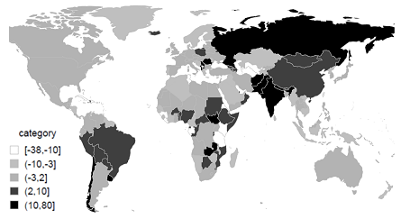
Fig. 2. Changes in global connectivity rates observed in various countries of the world from 2000 till present time

Importantly, even if a country experienced a decline in its position in the list of countries by global connectivity rates, it does not necessarily mean that its global connectivity rate per se declined too. Indeed, it can well be the case that the rate of this country's global integration grew during the period observed, but its growth was slower than in other countries (this is true for Denmark, Norway, Finland, Portugal, and some other countries).

Generally speaking, global connectivity rates have significantly increased since 2000 in the groups of countries where these rates ranged from 2 to 4, i.e., in the already rather well-integrated countries. On the contrary, only 27 per cent of countries with global connectivity rates less than 2 have increased their global integration since 2000. So, our results allow for a preliminary suggestion of a divergence in global connectivity rates among the well-integrated and the poorly-integrated countries; however, this suggestion requires further research to be either empirically corroborated or refuted.

ACKNOWLEDGMENT

This research has been supported by Russian Science Foundation project No 15-18-30063.

NOTE

¹ Data on confidence intervals estimations for global connectivity rates can be found at: URL: https://drive.google.com/open?id=0B2PD1YBY68PWcVVT M0tLY0 FRSG8.

REFERENCES

Anderberg, M. R. 1973. Cluster Analysis for Applications. New York: Academic Press.

A. T. Kearney Inc, 2001. Global Policy Group and Foreign Policy Magazine 2001. Measuring Globalisation. Foreign Policy 122: 56–65.

Dreher, A. 2006. Does Globalization Affect Growth? Evidence from a New Index of Globalization. Applied Economics 38 (10): 1091–1110.

Ernst & Young, 2012. Looking beyond the Obvious. Globalization and
New Opportunities for Growth. About the 2012 Globalization Index. URL: www.ey.com/GL/en/Issues/Drivinggrowth/Globalization---Looking-beyond-the-obvious---2012-Index.

Fortunato, S. 2010. Community Detection in Graphs. Physics Reports 486 (3–5): 75–174.

Luce, D., and Perry, A. 1949. A Method of Matrix Analysis of Group Structure. Psychometrika 14 (2): 95–116.

Martens, P., and Raza, M. 2008. An Updated Maastricht Globalization Index. ICIS Working Paper No. 08020. Maastricht: Maastricht University.

Martens, P., and Zywietz, D. 2006. Rethinking Globalization: A Modified Globalization Index. Journal of International Development 18 (3): 331–350.

Modelski, G. 2008. Globalization as Evolutionary Process. In Modelski, G., Devezas, T., and Thompson, W. R. (eds.), Globalization as Evolutionary Process: Modeling Global Change (pp. 11–29). London and New York: Routledge.

Raab, M., Ruland, M., Schonberger, B. et al. 2008. GlobalIndex – a Sociological Approach to Globalization Measurement. International Sociology 23 (4): 596–631.

Seidman, S. 1983. Network Structure and Minimum Degree. Social Networks
5 (3): 269–287.

Spath, H. 1980. Cluster Analysis Algorithms. Chichester: Ellis Horwood.

Vujakovic, P. 2010. How to Measure Globalization? A New Globalization Index (NGI). Atlantic Economic Journal 38: 237. URL: https://doi.org/10.1007/ s11293-010-9217-3.

Zinkina, J., Korotayev, A., and Andreev, A. 2013. Measuring Globalization:
Existing Methods and Their Implications for Teaching Global Studies and Forecasting. Campus-Wide Information Systems 30 (5): 321–339.

Appendix

Global Connectivity Rates for Top-50 Most Integrated Countries of the World, 2000–2004, 2005–2009, and 2010–2017

Rank	Country	Trade in goods	Trade in services	FDI	Migration	Total
1	United Kingdom	1.000	1.000	1.000	1.000	4.000
2	United States	1.000	1.000	1.000	1.000	4.000
3	Germany	1.000	1.000	1.000	1.000	4.000
4	Italy	1.000	1.000	1.000	1.000	4.000
5	France	1.000	1.000	1.000	1.000	4.000
6	Spain	0.999	1.000	1.000	0.996	3.995
7	Netherlands	1.000	1.000	1.000	0.982	3.982
8	Switzerland	0.999	0.997	0.999	0.985	3.980
9	Belgium	1.000	1.000	0.999	0.973	3.973
10	China	1.000	0.988	0.975	0.996	3.959
11	Japan	0.999	0.988	0.984	0.974	3.944
12	Canada	0.993	0.969	0.980	1.000	3.943
13	Russia	0.999	0.978	0.958	0.983	3.919
14	Ireland	0.980	1.000	0.987	0.940	3.907
15	Sweden	0.992	0.980	0.979	0.943	3.895
16	Australia	0.997	0.931	0.967	0.995	3.890
17	Poland	0.991	0.942	0.940	0.998	3.872
18	South Korea	0.998	0.948	0.934	0.971	3.852
19	Austria	0.986	0.944	0.954	0.964	3.848
20	Denmark	0.981	0.979	0.962	0.901	3.823
21	India	0.998	0.920	0.890	0.989	3.796
22	Brazil	0.994	0.833	0.985	0.978	3.790
23	Singapore	0.998	0.968	0.972	0.842	3.780
24	Norway	0.986	0.896	0.969	0.906	3.757
25	Hong Kong	0.998	0.974	0.942	0.837	3.751
26	Turkey	0.994	0.901	0.866	0.980	3.742
27	Hungary	0.976	0.880	0.897	0.939	3.692
28	Finland	0.976	0.937	0.909	0.865	3.687
29	Portugal	0.959	0.876	0.847	0.982	3.663
30	Czech Republic	0.986	0.892	0.846	0.922	3.646
31	Luxembourg	0.879	0.989	1.000	0.720	3.588
32	Greece	0.950	0.929	0.712	0.970	3.560
33	South Africa	0.983	0.733	0.882	0.945	3.542
34	Thailand	0.997	0.726	0.832	0.938	3.493
35	Malaysia	0.997	0.693	0.835	0.946	3.471
36	Romania	0.964	0.803	0.700	0.988	3.456
37	Chile	0.956	0.743	0.843	0.888	3.430
38	Israel	0.966	0.755	0.718	0.963	3.402
39	Mexico	0.993	0.719	0.814	0.872	3.398
40	Bulgaria	0.922	0.729	0.678	0.951	3.281
41	New Zealand	0.940	0.737	0.617	0.938	3.232
42	Slovakia	0.964	0.758	0.670	0.837	3.229
43	Indonesia	0.996	0.632	0.624	0.969	3.222
44	Cyprus	0.831	0.735	0.800	0.819	3.185
45	Ukraine	0.960	0.591	0.597	0.981	3.129
46	Philippines	0.963	0.583	0.542	0.985	3.073
47	Argentina	0.961	0.587	0.588	0.929	3.066
48	Croatia	0.888	0.745	0.539	0.855	3.026
49	Pakistan	0.938	0.638	0.366	0.983	2.925
50	Egypt	0.957	0.673	0.324	0.968	2.922

Note: For a full list of countries and their global connectivity indices and ranks see: URL: https://drive.google.com/open?id=0B2PD1YBY68PWN0FaRF9faUVtR1k.