The Effect of Financial Independence of Indian Women on Their Marriage Decisions

Authors: Jain, Sidhant; Chuphal, Bhawna; Shakarad, Mallikarjun N.
Journal: Social Evolution & History. Volume 22, Number 1 / March 2023

DOI: https://doi.org/10.30884/seh/2023.01.06

Sidhant Jain, Institute for Globally Distributed Open Research and Education (IGDORE); University of Delhi, North Campus, Delhi

Bhawna Chuphal, University of Delhi, North Campus, Delhi

Mallikarjun N. Shakarad, University of Delhi, North Campus, Delhi; Jawaharlal Nehru Centre for Advanced Scientific Research, Govt. of India, Bengaluru

Mate choice is a complex process in all sexually reproducing animals. In case of humans, this process becomes more intense since social, economic and cultural norms influence this decision. A common observation among different human cultures is that the men prefer younger women because of their fertility whereas women prefer an older man who might have attained social status and economic stability, thus maximizing the Darwinian fitness of both the individuals. In this study, we analyzed the influence of financial independence of Indian women, which they attained as a result of a boom in the IT sector, on their age of marriage and choice of groom (in terms of grooms' age). Our results show that financially independent Indian women of the post-IT boom period, preferred to marry late in their lives with a groom around their own age. On the contrary, men both in the pre- and post-boom times sought for a younger bride.

Keywords: evolution, Darwinian fitness, financial independence, marriage pattern, the IT boom.

1. INTRODUCTION

In all the monogamous sexually reproducing species, mate choice is a vital decision, as the mate quality is associated with the fitness benefits accrued to the pair in the form of better quality progeny, improved social status, provisioning of resources, protection from harassment and such other coercive acts by conspecifics. On the other hand, poor choice can inflict costs such as sexually transmitted diseases, high mutation load in the genetic material, reputational damage and abandonment (Buss 1989; Buss and Schmitt 2019). These costs and benefits continue to exert selection pressure in every generation of sexually reproducing species.

Several traits have evolved as indicators of the mate quality in different species. In peacock, the length of the train and number of eyespots is shown to be a good indicator of the male quality (Petrie et al. 2009; Yorzinski et al. 2013). In many species, males offer nuptial gift to the female in order to be accepted as a mate (Miller 1998). However, in the case of humans, a species which is culturally and socially complex, the choice of mate is influenced by many other considerations, as a result of which humans have evolved multiple mating strategies involving unique features. Our evolved preferences and forms of mate competition are complex and differ in some key aspects from those of other known sexually reproducing species (Buss and Schmitt 2019).

The near permanent association between a woman and a man, quite often solemnized in marriage in most societies, is established invariably between a relatively younger woman and a man who is often older than the woman. The preference for younger women is suggested to be due to her high reproductive value and women's preference for men older than themselves is suggested to be due to their accumulated wealth, social status and economic stability. Together, the age preference of two sexes for partners in opposite direction may yield fitness benefits for both and this might be evolutionarily selected (Buss 1989; Kenrick and Keefe 1992; Fieder and Huber 2007; Helle et. al. 2008).

In the past decades, many studies have attempted to examine the impact of industrialization and urbanization on the lives of people in many developing countries. The processes of mate selection often vary widely depending on the society, from those completely decided by the elders of the family without the active participation of the potential marriage partners to limited ‘freedom of choice’ in India. In the United States of America and many other Western countries, the possible explanations for partner selection are classified into individual and socio-cultural explanations (Siddiqi and Reeves 1989). In the late 1990s, globalization unveiled a potential employment opportunity for Indian women in Information Technology (IT) sector offering an opportunity to be financially independent (Bhattacharyya and Ghosh 2012), thus liberating them from the strong patriarchal control and suppression. 

Prior to the IT-boom period, a large majority of women in India married with negligible communication, if any at all, with their to-be-spouses as the alliance were traditionally forged by the parents of the prospective bride and groom. This was perhaps due to strong patriarchal society and to an almost complete financial dependence of women. In a completely contrasting scenario, many women became able to achieve financial independence due to the IT explosion that offered jobs outside their homes. Even though women preserve their traditional care-giving role, they continue to climb the ladder of increasing financial independence.

Moreover, an increasing number of women pursue traditionally male-dominated careers, closing the gender gap in earnings. A few researchers have investigated how women's earning capacity is tied to their mate preferences (Buss 1989; Feingold 1992; Kenrick et al. 1990). Women who have greater focus on career with high income tend to emphasize on potential mates' resource-acquisition ability; so such wo-men occupy high professional position and may look for partner with even higher professional position and status. It seems that the better economic prospects of women lead to the higher standards for earning capabilities in their mate (Zhang et. al. 2014).

In the present study we assessed whether financial independence of Indian women led to their active participation in the decision making process of choosing their potential marriage partner. In addition, we discuss implications of financial independence on mate choice in Indian population.

2. METHODS

2.1 Data Collection

The matrimonial advertisements (advertisements given by men or women for a potential marriage partner) published in Sunday edition of three different popular newspapers of India were used to collate and classify the data as shown in Table 1. The different newspapers used have a similar coverage and readership. All the published advertisements which clearly indicated the age of a focal bride/ groom and the expected age range of potential partner were chosen irrespective of religion, caste, profession, income and/or any other considerations. Hence, any bias arising because of these considerations was potentially avoided.

The advertisements which clearly mentioned a case of second marriage (SM) were marked and all others were treated as first marriage. Though information on parameters like height and salary was collected, however, as information on these parameters was not uniformly available, the effects of these factors could not be assessed.

India witnessed an IT boom in the early 2000s. In 2000/01, the Indian IT sector exported software and related services worth $6.4 billion which was nowhere close to the value of exported services of the 1980s or 1990s. A growth of 55 per cent was witnessed in the IT software and services industry in 2000/01 (Kapur 2002). Hence, the period after this significant feat was considered as the post-IT boom period whereas the period before this was labeled as that of the pre-IT boom.

The IT sector played a significant role in women empowerment from the early 2000s as it provided a potential employment opportunities for women in organized sector and made them financially independent (Bhattacharyya and Ghosh 2012). Gradually, Indian women preferred to work outside home to limit the dependency on their families as well as improve upon their social status (Kelkar and Nathan 2002). Hence, the period of 2005–2009 was chosen to collect data on the IT sector since this time period provided many employment opportunities to women making them financially independent throughout major cities of India (Bhattacharyya and Ghosh 2012).

Most studies published in psychological and behavioral journals obtained 96 per cent of their data from ‘WEIRD’ population, an acronym used for Western, Educated, Industrialized, Rich and Democratic, which represents only 12 per cent of the human population of the world (Henrich et al. 2010). In our view, the data used in this work represents individuals who perhaps belong to the middle-class society consisting of many different castes, religions, financial status and political orientations as the data is drawn from pan-Indian population. However, the educational qualifications although different were not variable across the two time zones.

Further, a questionnaire was prepared to collect primary data regarding the age of women, educational qualification and financial independence at marriage from those who had married during the pre-IT boom period and in the post-IT boom period, latter being collected from women working in the IT field. The responses were collected only from women responders. This questionnaire was send to 40 women in each group. Thirty-two women responded for the pre-IT period and thirty-one responded for the post-IT period. The questions covered age and educational qualifications of women at marriage, choice and active participation in marriage decisions, age of spouse at marriage and financial independence of women at marriage. Data on active participation, final decision to marry a particular individual and on financial independence were extracted from the questionnaire-responses.

Table 1

Data collection methodology

Timeline	Data years	Newspapers	Parameters
			Focal person (Bride/Groom)	Potential partner
Pre-IT period (2000 and before)	1994, 1998, 1999, 2000	The Tribune1 The Indian Express2	Age, height*, salary*	Acceptable age range, height* and salary*
Post-IT period (after 2000)	2005–2009	The Times of India3	Age, height*, salary*	Acceptable age range, height* and salary*

Notes: ^* if mentioned

¹ https://www.tribuneindia.com/2014/forms/archive.htm.

² https://news.google.com/newspapers?nid=P9oYG7HA76QCanddat=19940101andprintsec=frontpageandhl=en.

³ http://epaper.timesofindia.com/Default/ClientEpaperBeta.asp?skin=pastissues2andenter=LowLevel.

2.2 Data Management and Statistical Analyses

All the statistical analyses were performed using GraphPad Prism 6 software and the graphs were made using Microsoft Excel software. For the pre-IT period, data from four years was pooled, generating 52 and 91 data points for brides and grooms respectively. Similarly, five year data was pooled for the post-IT period timeline generating 1120 and 1426 data points respectively. Further, for the post-IT period we succeeded to extract 71 and 74 second marriage data points for brides and grooms respectively.

The analysis of advertised age and age range of partners sought. The data was tabulated according to the age of the focal individual and the age range of the partner sought during the pre-IT and post-IT period. All statistical comparisons were made between the pre-IT and post-IT data, and the first and second marriage of the post-IT data. From this primary data the average and modal age of the focal individual, the average age of the partner sought and the average acceptable age difference between partners were ascertained (see Appendix 1 for Index Table). In addition, we also ascertained the average age range sought by a focal individual age. For this, the average minimum age limit and average maximum age limit for each focal age were calculated (see Appendix 1 for calculation methodology). The age differences between the focal individuals and the partners sought were also calculated by subtracting the age of focal individual from minimum, average and maximum age of partner sought. Further, the N value for the post-IT period data was nearly 20 times larger than for the pre-IT period data. In order to make sure that the data size itself does not influence the results, additional statistical tests were carried out (Appendix 2).

The t-tests. The average age of the focal individuals, the average age of partners sought, the age difference between the focal individual and the prospective partner and the regression slopes were compared between pre-IT and post-IT period using student's t-test. The details of all the unpaired t-tests performed in this study are listed in Table 2.

Table 2

List of different parameters compared using t-tests

Groups	Parameter
Group-1. Bride	1. Age of giving advertisement for first marriage (Pre-IT vs. post-IT boom period). 2. Minimum age limit difference of prospective partner at first marriage (Pre-IT vs. post-IT period). 3. Maximum age limit difference of prospective partner at first marriage (Pre-IT vs. post-IT period). 4. Minimum age limit difference of prospective partner at first marriage vs. second marriage (the post-IT period). 5. Maximum age limit difference of prospective partner at first marriage vs. second marriage (the post-IT period). 6. Age of marriage of women in pre- and post-IT boom period (from questionnaire responses)
Group-2. Groom	All the five tests as above
Group-3. Bride vs. Groom	Age at which a bride starts giving an advertisement for marriage as compared to groom for both the timelines
Group-4. Regression	t-statistic used to compare the pre- and post-IT regression slopes obtained by taking age of focal individual as independent variable and differences between the ages as dependent variable (for data collected using newspapers and from questionnaire-responses)

Regression. The regression analysis was carried out with age of focal individual as independent variable and the difference at lower age limit, upper age limit and mean age of the acceptable partner as dependent variable. The slope of the pre-IT and post-IT data were compared using t-statistic (Zar 2014) to ascertain any effect of economic independence of the women on the preferred and acceptable age of the groom.

Furthermore, summary data from questionnaire-responses of women from the pre-IT and post-IT period were subjected to two-proportion Z test.

3. RESULTS

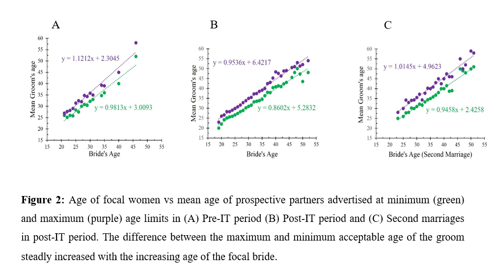
There was a significant increase in the age at which the brides advertised for first marriage during the post-IT time period compared to their counter parts in the pre-IT time period (Table 3). During the pre-IT period, women used to start giving advertisement for first marriage when they were 27.12 ± 5.04 years old (Modal Value: 22), while those during the post-IT period advertised at an average age of 28.88 ± 4.89 (Modal Value: 25) (Fig. 1A). The acceptable age range of the men increased with increasing age of the focal women (Fig. 2A and 2B). In addition, during 2004–2009 phase (Fig. 2C), for second marriages women preferred a steady increase in age range till 40 years of age after which the preferred age range showed more variation than the steadily increasing pattern.

Table 3

Results of the T-test analyses

Group	Parameter (as per Table 2)	t-value	Df	p value
Bride	Age of giving advertisement for first marriage (pre-IT vs. post-IT period)	2.512	1170	0.0122**
	Minimum age limit difference of prospective partner at first marriage (pre-IT vs. post-IT)	4.584	1170	<0.0001***
	Maximum age limit difference of prospective partner at first marriage (pre-IT vs. post-IT)	2.898	1170	0.0038**
	Minimum age limit difference of prospective partner at first marriage vs. second marriage.	2.125	1189	0.0338*
	Maximum age limit difference of prospective partner at first marriage vs. second marriage.	2.187	1189	0.0049**
	Age of marriage of women in pre- and post-IT boom period (from questionnaire responses)	13.087	62	<0.0001***

Table 3 (continued)

Group	Parameter (as per Table 2)	t-value	Df	p value
Groom	Age of giving advertisement for first marriage (Pre-IT vs. post-IT period)	2.690	1515	0.0072**
	Minimum age limit difference of prospective partner at first marriage (Pre-IT vs. post-IT)	0.485	1515	0.6276
	Maximum age limit difference of prospective partner at first marriage (Pre-IT vs. post-IT)	2.038	1515	0.0417*
	Minimum age limit difference of prospective partner at first marriage vs. second marriage.	15.010	1498	<0.0001***
	Maximum age limit difference of prospective partner at first marriage vs. second marriage.	9.568	1498	<0.0001***
Bride vs. Groom	Pre-IT period	2.774	141	0.0063**
	Post-IT period	9.914	2544	<0.0001***

Notes:

^* Significant at 5 per cent;

^** Significant at 1 per cent;

^*** Significant at 0.01 per cent or higher.

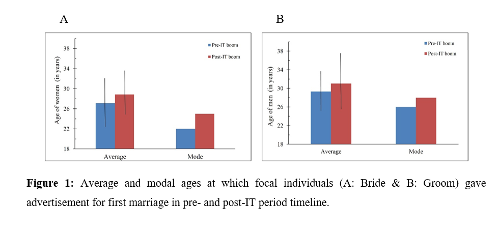
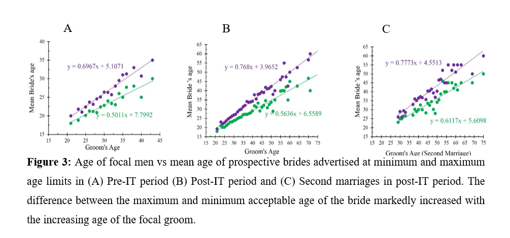
Further, there was a significant increase in the age at which the Indian grooms advertised for first marriage during the post-IT period as compared to pre-IT period (Table 3). Prior to the IT-boom period in India, men advertised for first marriage around an average age of 29.34 ± 4.28 (Modal Value: 26) while their counterparts during the post-IT period advertised around 31.05 ± 6.00 years of age (Fig. 1B) (Modal Value: 28). Men continued to advertise for younger women at all focal ages, though with an increase in their own age, the acceptable age range of women also widened both during the pre-IT (Fig. 3A) and post-IT (Fig. 3B) periods. Men advertising for second marriage during the post-IT period showed similar preference as the first marriage (Fig. 3C).

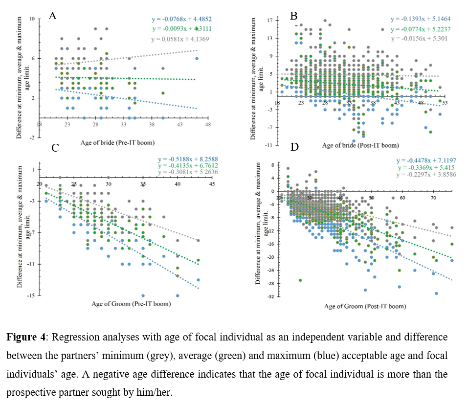
The regression analyses of the pre- and post-IT boom data with age of women as independent variable is shown in Table 4. When the slopes obtained in the regression analyses were compared by t statistic, there was a significant difference in the slopes for minimum (t = 4.69, p < 0.05), average (t = 4.63, p < 0.05) and maximum (t = 3.66, p < 0.05) acceptable ages (Fig. 4A and 4B). Similar regression analyses with age of men as the independent variable is shown in Table 5. The comparison of slopes obtained in the analyses of pre- and post-IT showed no significant difference for the minimum acceptable age (t = 1.87, p < 0.05). However, the slopes for average (t = 2.59, p < 0.05) and maximum (t =3.18, p < 0.05) acceptable age were significantly different (Fig. 4C and 4D).

Table 4

Regression analyses with age of women as independent variable

	Independent Variable	Dependent Variable	Slope Value	F Value	p Value
Pre-IT Boom Period	Age of women	Difference with min. acceptable age of men	–0.0768	3.071	0.0858
		Difference with average acceptable age of men	–0.0093	0.054	0.8167
		Difference with max. acceptable age of men	0.0581	1.636	> 0.2068
Post-IT Boom Period	Age of women	Difference with min. acceptable age of men	–0.1393***	150.4	< 0.0001
		Difference with average acceptable age of men	–0.0774***	53.76	<0.0001
		Difference with max. acceptable age of men	–0.0156	1.46	0.2271
*** Slope significantly different from zero (Significant at 0.01 per cent or higher)

Table 5

Regression analyses with age of men as independent variable

	Independent Variable	Dependent Variable	Slope Value	F Value	p Value
Pre-IT Boom Period	Age of men	Difference with min. acceptable age of women	–0.5188***	136.1	<0.0001
		Difference with average acceptable age of women	–0.4135***	150.6	< 0.0001
		Difference with max. acceptable age of women	–0.3081***	68.91	<0.0001

Table 5 (continued)

	Independent Variable	Dependent Variable	Slope Value	F Value	p Value
Post-IT Boom Period	Age of men	Difference with min. acceptable age of women	–0.4478***	2536	<0.0001
		Difference with average acceptable age of women	–0.3369***	1879	<0.0001
		Difference with max. acceptable age of women	–0.2297***	811.9	<0.0001
*** Slope significantly different from zero (Significant at 0.01 per cent or higher)

     

Note: Graphs can be checked online for colored version

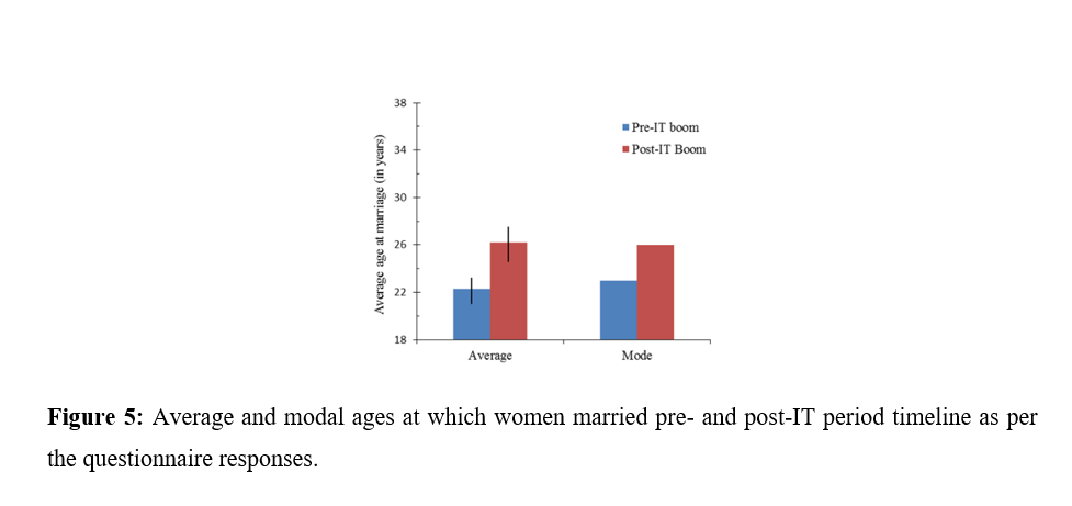
The primary data collected using questionnaire (Fig. 5) showed that the Indian women married at a significantly older age in the post-IT boom than pre-IT period (t = 13.087, p < 0.0001, Table 3).

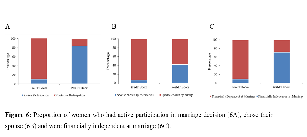
Two-proportion z-test on the number of individuals actively participated in the decision making process, final decision on acceptance of a specific individual as life-partner and financial independence at the time of marriage showed significant difference between pre-IT and post-IT period brides. Significantly higher number of women were actively involved in choosing their life-partner in the post-IT period compared to pre-IT period (z = 5.931, p < 0.00006; Fig. 6A). Similarly, significantly higher number of individuals took the final decision on their life-partner in the post-IT period compared to pre-IT period (z = 3.70, p < 0.00042; Fig 6B). Further, significantly higher number of individuals were financially independent in the post-IT period compared to pre-IT period (z = 4.996, p < 0.00006; Fig. 6C).

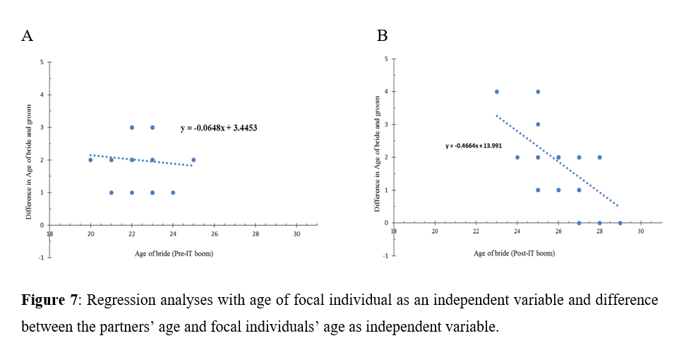
     The regression analysis (Fig. 7A and B) with age of women as independent variable and difference in age of spouse as independent variable generated non-significant non-zero slope (slope= –0.06478, F= 0.2449, p= 0.6243) in pre-IT period. In post-IT period, a significantly non-zero negative slope was obtained (slope= –0.4664, F= 9.826, p= 0.0039). The t-statistic which was used to compare the slopes of two timelines showed a significant difference (t = 2.113, p < 0.05).

 Before the IT-boom, a considerable number of women (73 per cent) gave their height specifications in the advertisement but none of them asked for any height specification for their prospective groom. Similarly, 79 per cent of males in the pre-IT boom specified their height and of the total males in the data set, only 11 per cent requested for specific height parameters from their prospective brides. There was a shift in this trend in post-IT boom period as 86.60 per cent of women and 85.62 per cent of men specified their height in the matrimony advertisement but about 15 per cent of total women and 31 per cent of total men asked for height specifications from their prospective partners.

4. DISCUSSION

Many women became financially independent and secure after the Information Technology growth in India (Bhattacharya and Ghosh 2012), thus releasing them from their dependence on men for their daily needs. The financial independence in turn enabled them to become active participants in the decision making process prior to entering into a wedlock as against the decision being exclusively taken by the parents, grandparents and other elders prior to the IT revolution (Fig. 6A and B). Thus, financial independence released the Indian women from the clutches of patriarchy and lead to their liberation, albeit partially. Further, financial independence in turn resulted in women deciding to delay marriages till they were about 25 years old (modal age at which advertisements were issued in daily newspapers) as against 22 years old in the pre-IT revolution period.

Further, women in the post-IT boom period also started asking for height specifications from their prospective partners which was not the case during the pre-IT boom period. Though the males specified their height and asked for specific height from their prospective partners in both the timelines but this was not the case for women in the pre-IT boom period.

The average age of Indian women at the time of marriage in the pre-IT and post-IT periods from the primary data (questionnaire-responses, Fig. 5) closely reproduces the data obtained from Sunday newspapers' matrimonial advertisements. The educational qualifications of women during the pre-IT and post-IT periods, as evidenced in the responses gathered as well as from the newspaper matrimonial advertisements were similar (all were graduates, except for one case when the bride passed 12^th standard) and hence it is safe to assume that education per se did not alter the results and inferences of this study. It is important to note that shifting marriage to a later age occurs despite the presumed decline in their fertility with increasing age (Richardson et al. 1987; Faddy et al. 1992; The American College of Obstetricians and Gynecologists, 2014). The financial freedom coupled with the advances in medical field with respect to fertility treatment, gamete storage for later conception and realization of Darwinian fitness through surrogacy (Borovecki et al. 2018) could have led to delaying marriages itself.

Attaining Darwinian fitness is the ultimate aim of every extant species. The desire of men for younger women seems to be strongly inherent in human societies across ethnic groups. Similar to situation in Western countries, Indian men prefer younger women (Buss 1989; Eichler 2012). The idea of the preference of younger women appears to be correlated with the female fertility (Fieder and Huber 2007; Helle et al. 2008). Before the IT-period, the difference between the age of groom and the expected median age of bride was relatively more since women were willing to get married at a younger age. However, after the IT-boom period, the financial independence and career centric women, perhaps, narrowed the age gap (Fig. 2). The narrowing in the observed age gaps is significant, as shown by t-tests (test 2 and 3 in Table 2).

The women's financial independence did not have any influence on the ‘younger bride seeking’ behavior of men as shown by insignificant difference obtained in the t-test (Table 3) comparing the acceptable age difference at lower limit of brides by the prospective grooms in the two time lines. However, the minimum age difference significantly decreased in the post IT-period suggesting that men were also marrying relatively older women in the post-IT period. This possibly is due to the women focusing on career during the initial period of employment as against starting a family as in the pre-IT period.

Women preferred a potential partner who is about four to five years older but at least one to two years older at most focal ages in both the timelines (Fig. 2A and 2B). The preference for older men seems to be strongly imprinted as fitness of women in union with older men is likely to be higher due to accumulated wealth, economic stability and social status of older men as against the younger ones (Buss 1989) besides emotional maturity of older men. The expectation of the men remained similar irrespective of the first or second marriage (Fig. 3) thus suggesting a strong inherent desire in men for women younger than themselves as marriage partners.

This study shows that Indian women start looking for a partner at an earlier age as compared to men. This trend was consistent across the both timelines as shown by significant difference in the t-test com-paring the age at which men and women advertised during the two timelines (Table 3). This possibly could be due to the underlying knowledge that they would not be able to beget children due to declining fertility with increasing age (Richardson et al. 1987) although the easy and affordable access to fertility clinics due to women's financial independence ushered in by the IT revolution points towards other reasons like hormonal influence on appearance of individuals.

Analysis of the data by considering 45 years as the maximum age limit of the women either as focal individual or the accepted upper age of the bride by men revealed that as the women's age increased, the age range of the men widened although they were willing to accept men younger than themselves (Fig. 3A and 3B). The acceptance of younger men could be an outcome of a desire for emotional support brought about by companionship and or a desire to fulfill the sexual urges. As humans are social animals, companionship is an important factor for them (Rook 1987). Men seemed to desire women of ~ 25 years of age irrespective of their own age as indicated by the regression slopes obtained with increasing age of the focal men (Fig 4C and 4D). The prefe-rence might be inherent due to fixated view of women's physical attractiveness at younger ages rather than their fertility (Little et al. 2011; Price et al. 2013). Our results not only support previous studies (Buss 1989; Eichler 2012), but also the results obtained in a similar previous study which employs a strategy very similar to ours (Wieder-man 1993).

The significant differences in the acceptability of marriage partners by women and men of Indian population show sexual dimorphism. This study demonstrates the active participation of women in decision-making with respect to their marriage after the IT-boom period as against passive participation during pre-IT period where the decision about their marriage were imposed on them by the patriarchal society primarily due to their financial dependence (Fuller and Narasimhan 2008; Desai and Andrist 2010; South et al. 2016).

5. CONCLUSION

The development of the information technology sector in India resulted in employment generation especially for younger women thus making them financially independent that in turn socially enabled them and liberated them from the clutches of patriarchal society with respect to the choice of life partners. Thus, they became active participants in the decision making process that resulted in asking for height specifications from their prospective partners, narrowing of the age gap between the marriage partners on addition to delaying marriage to later years (that indirectly facilitated passive decision making with respect to reproduction).

As in other societies, Indian women prefer men who are older than themselves as marriage partners due to the economic, social, and perhaps, emotional stability provided by older men as against younger men. However, with increase in their own age they exhibited acceptance to marry younger men perhaps for the purpose of compani-onship even if it is uncertain. Men, on the contrary, prefer younger women even with the progression in their own age which seems to be evolutionary conserved in order to ensure Darwinian fitness besides suggesting sexual dimorphism among the two genders with respect to age preference of potential marriage partners.

6. DECLARATIONS

Funding sources: The present study was not funded by any funding institute.

Conflict of Interests: The authors declare that they have no conflict of interest.

Ethics approval: Not Applicable.

REFERENCES

Bhattacharyya, A., and Ghosh, B. N. 2012. Women in Indian Information Technology (IT) Sector: A Sociological Analysis. IOSR Journal of Humanities and Social Science (JHSS), 3 (6): 45–52.

Borovecki, A., Tozzo, P., Cerri, N., and Caenazzo, L. 2018. Social Egg Freezing under Public Health Perspective: Just a Medical Reality or a Women's Right? An Ethical Case Analysis. Journal of Public Health Research, 7(3): 1484.

Buss, D. M. 1989. Sex Differences in Human Mate Preferences: Evolutionary Hypotheses Tested in 37 cultures. Behavioral and Brain Sciences, 12 (1): 1–49.

Buss, D. M., and Schmitt, D. P. 2019. Mate Preferences and Their Behavioral Manifestations. Annu Rev Psychol, 70: 77–110.

Desai, S., and Andrist, L. 2010. Gender Scripts and Age at Marriage in India. Demography, 47 (3): 667–687.

Eichler, M. 2021. Marriage in Canada. The Canadian Encyclopedia. https://www.thecanadianencyclopedia.ca/en/article/marriage-and-divorce

Faddy, M.J., Gosden, R.G., Gougeon, A., Richardson, S.J., and Nelson, J. F. 1992. Accelerated Disappearance of Ovarian Follicles in Midlife: Implication for Forecasting Menopause. Hum Reprod.10: 1342–6.

Feingold, A. 1992. Gender Differences in Mate Selection Preferences: A Test of the Parental Investment Model. Psychol Bull, 112 (1): 125–139.

Fieder, M., and Huber, S. 2007. Parental Age Difference and Offspring Count in Humans. Biology Letters 3: 689–691.

Fuller, C. J., and Narasimhan, H. 2008. Companionate Marriage in India: The Changing Marriage System in a Middle-Class Brahman Subcaste. Journal of the Royal Anthropological Institute (N.S.), 14: 736–754.

Helle, S., Lummaa, V., and Jokela, J. 2008. Marrying Women 15 Years Younger Maximized Men's Evolutionary Fitness in Historical Sami. Biology Letters, 4: 75–77.

Henrich, J., Heine, S.J., and Norenzayan, A. 2010. Most People are not WEIRD. Nature. 466 (7302): 29.

Kapur, D. 2002. The Causes and Consequences of India's IT Boom. India review 1 (2): 91–110.

Kelkar, G., and Nathan, D. 2002. Gender Relations and Technological Change in Asia. Current Sociology, 50 (3): 427–441.

Kenrick, D. T., and Keefe, R. C. 1992. Age Preferences in Mates Reflect Sex Differences in Human Reproductive Strategies. Behavioral and Brain Sciences, 15: 75–133.

Kenrick, D. T., Sadalla, E. K., Groth, G., and Trost, M. R. 1990. Evolution, Traits, and the Stages of Human Courtship: Qualifying the parental Investment Model. J Pers, 58 (1): 97–116.

Little, A. C., Jones, B. C., and DeBruine, L. M. 2011. Facial Attractiveness: Evolutionary Based Research. Philosophical Transactions of the Royal Society of London. Series B, Biological sciences, 366 (1571): 1638–1659.

Miller, G. 1998. A Review of Sexual Selection and Human Evolution: How Mate Choice shaped Human Nature. ESRC Centre on Economics Learning and Social Evolution, ELSE working papers.

Petrie, M., Cotgreave, P., Pike, T.W. 2009. Variation in the Peacock's Train Shows a Genetic Component. Genetica, 135 (1): 7–11.

Price, M. E., Pound, N., Dunn, J., Hopkins, S., and Kang, J. 2013. Body Shape Preferences: Associations with Rater Body Shape and Sociosexuality. PloS one, 8 (1): e52532.

Richardson, S. J., Senikas, V., and Nelson, J. F. 1987. Follicular Depletion during the Menopausal Transition: Evidence for Accelerated Loss and Ultimate Exhaustion. J. Clin. Endocrinol. Metab., 65: 1231–1237.

Rook, K. S. 1987. Social Support versus Companionship: Effects on Life Stress, Loneliness, and Evaluations by Others. Journal of Personality and Social Psychology, 52 (6): 1132–1147.

Siddiqi, M. U., and Reeves, E. Y. 1989. A Comparison of Marital Preference of Asian Indians in Two Different Cultures. International Journal of Sociology of the Family, 19 (1): 21–36.

South, S. J., Trent, K., and Bose, S. 2016. Demographic Opportunity and the Mate Selection Process in India. J Comp Fam Stud, 47 (2): 221–246.

The American College of Obstertricians and Gynecologists. 2014. Committee opinion 589: Female age-related fertility decline, 123: 719–721.

Wiederman, M. W. 1993. Evolved Gender Differences in Mate Preferences: Evidence from Personal Advertisements. Ethology and Sociobiology 14: 331–352.

Yorzinski, J. L., Patricelli, G. L., Babcock, J. S., Pearson, J. M., and Platt, M. L. 2013. Through Their Eyes: Selective Attention in Peahens During Courtship [published correction appears in J Exp Biol. Nov 15; 216 (Pt 22):4310]. J Exp Biol. 216 (Pt 16): 3035–3046.

Zar, J. H. 2014. Biostatistical Analysis. 5^th edition. Pearson Education Limited, England.

Zhang, H., Teng, F., Chan, D. K., and Zhang, D. 2014. Physical Attractiveness, Attitudes toward Career, and Mate Preferences among young Chinese Women. Evol Psychol, 12 (1): 97–114.

Appendix

Appendix 1

Table 6

Index Table defining various terms used in the text

Index Table
Age of focal individual (in years)	The age at which a man or woman (prospective groom/ bride) advertises for marriage
Minimum age limit (in years)	The minimum age of partner sought by a focal individual
Maximum age limit (in years)	The maximum age of partner sought by a focal individual
Average (mean) age limit (in years)	Average of minimum and maximum age limit
Average minimum and maximum age limit (in years)	Calculated for each focal age. For example, if the focal individuals are grooms of age 25, then, all the data points for 25 year old grooms were selected and mean values at advertised minimum and maximum age limits of the brides sought were calculated as shown in example below
Mean minimum age limit difference	Average of (Minimum Age limit advertised by focal individuals – Age of focal individual)
Mean of average age limit difference	Average of (Mean Age limit calculated – Age of focal individual)
Mean maximum age limit difference	Average of (Maximum Age limit advertised by focal individual – Age of focal individual)

Table 7

Example showing calculation of average age limit
and average minimum and maximum age limit

Age of Groom (focal individual) in years	Minimum age limit of bride sought (in years)	Maximum age limit of bride sought (in years)	Average (mean) age limit of bride sought (in years)	Average minimum age limit of brides sought (in years)	Average maximum age limit of brides sought (in years)
25	20	21	20.50	22	23
25	22	24	23
25	24	24	24
26	23	24	23.50	23	24.5
26	23	25	24

Appendix 2

In order to ensure that the relative huge amount of data points in post-IT period timeline don’t influence our result, we carried out stratified sampling within the focal age of either the bride or the groom and obtained post-IT data size similar to that of pre-IT data. Two data sets each for brides and grooms of post-IT period timeline with reduced data points were generated and t-tests (1–3 of Table 2) were carried out. Hence we had 12 sets of data on which we applied t-tests.

11 of these 12 t-tests generated the same results of significance or insignificance as obtained with the actual data of post-IT period. Only one t-test applied on age of bride and maximum age difference of prospective partner, became slightly insignificant. Hence, it can be concluded that the significant differences obtained are not a result of the difference between the data points as shown by stratified random sampling of post-IT period data.