Another, Simpler Look: Was Wealth Really Determined in 8000 BCE, 1000 BCE, 0 CE, or Even 1500 CE?

Almanac: History & Mathematics:Trends and Cycles
Abstract
Olsson and Hibbs (2005) and Comin, Easterly, and Gong (2010) make persuasive theoretical and empirical cases for the persistence of early biogeographical and technological advantages in predicting the distribution of national economic wealth. However, these results are challenged with an examination of sixteen observations on economic complexity, GDP per capita, and city size spanning as much as ten millennia and eight to eleven regions. The regional complexity / wealth hierarchies are relatively stable only for finite intervals. Early advantages, thus, have some persistence but do not linger indefinitely. The rich do not always get richer or even stay rich, and the poor sometimes improve their standings in the world pecking order dramatically. Early advantages are important but need to be balanced with the periodic potential for overriding them.
Keywords: economic growth, early advantage, biogeographical advantage, technological advantage, city size, societal complexity.
Introduction
We live in an era fraught with the potential for tectonic changes in relative economic positioning. The United States, long the leader in technological innovation and economic growth, is combating symptoms of relative decline and an increasingly visible challenge from China, a state emerging rapidly from a long period of relative underdevelopment. Japan, thought to be the most likely economic challenger to the United States less than two decades ago, is mired in relative stagnant growth and facing a serious population aging problem. Russia, once a challenger to the United States, experienced an economic meltdown when the Soviet Union fragmented. But Russia is re-emerging as an economic competitor of sorts by exploiting the sale of raw materials. A state adjacent to China, India, equally populous, seeks to catch up and surpass China. The region that the United States once overtook, Western Europe, remains affluent but is confronted currently with the prospect of the world's one successful regional integration experiment breaking up. Throughout all of these potential changes in the making, a large number of states remain poor and have few prospects for any change in the near, or perhaps distant, future.
It is hardly surprising, then, that the question of how economies grow fast and slow and why some economies get ahead of others while others fall back is popular.[1] Many of the arguments that have surfaced focus on more recent developments and yet many of these remain untested empirically. Olsson and Hibbs (2005) and Comin, Easterly, and Gong (2010) are remarkable exceptions to these generalizations. Not only do their studies encompass thousands of years, they go to some lengths to test their perspective on long-term economic growth. Olsson and Hibbs find that Diamond's (1997) argument, predicated on the technological advantages associated with diffusion possibilities linked to continental axes and the distribution of edible plants and large mammals prior to the advent of agriculture, predict well to current national incomes. The strong implication is that the world's distribution of income was determined even before the advent of agriculture. Comin, Easterly, and Gong find that technological adoption in 1500 CE predicts well to national income in the current period and that knowing about the distribution of technology in 1000 BCE and 0 CE predict respectively to technological distributions in 0 CE and 1500 CE. They conclude that the world's distribution of technology has been quite persistent. Wealth distributions, to the extent that they are predicated on technological attainments, were not strictly determined in 1000 BCE but the extent of path dependency is quite strong. Areas that have been technologically ahead in the past tend to continue to be technologically ahead in the present.
Ambitious and largely unprecedented analyses, however, are likely to be characterized by various empirical and design problems. Attempting to capture changes in economic development over thousands of years is never easy or straightforward. Assuming then that there will always be some problems, the question is whether the problems appear to strongly influence the outcome. In this case, the answer is that assumptions made in the research design appear to have biased the conclusions significantly. We do not dispute Olsson and Hibbs (2005) and Comin et al.'s (2010) specific findings as much as what we should make of them. If the central question is whether technological differences persist over long periods and the answer lies in the affirmative, there are at least several major caveats that need to be advanced based on the long-term analysis of uneven economic development. By more than tripling the length of the Comin et al.'s examination (from three millennia to ten millennia), expanding the number of observations (to sixteen across the ten millennia), changing the unit of analysis (from contemporary states to regions), and simplifying the indicators relied upon (substituting a different index of complexity for prehistorical times and gross domestic product per capita and city size for historical times), a more comprehensive picture of long-term development emerges. The persistence of earlier technological advantages does not disappear. On the contrary, it is quite evident. But so too are major departures from persistence. We should not emphasize one dimension over the other. Instead, we should strive to integrate both dimensions in understanding long-term changes.
The Persistence Analyses
Our problems with the two earlier studies differ by study. The Olsson and Hibbs (2005) study develops, elaborates, and operationalizes Diamond's (1997) argument well.[2] Fig. 1 summarizes their theory and empirical model. Favorable climate, larger continental size, and an east-west axis that permits diffusion of seeds, animals, and technology increases the availability of plants and animals that are suitable for agriculture. The greater is the availability of plants and animals, the greater is the opportunity to experiment with agrarian techniques. Agrarian and industrial revolutions should occur earlier in such areas than in less favored regions. The earlier is the timing of agrarian and industrial revolutions, the greater should be the contemporary level of income per capita.
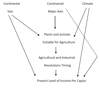
Fig. 1. Logical structure of Olsson and Hibbs' theory (2005: 928)
One can balk at various aspects of the Diamond argument or not but our main criticism of the Olsson and Hibbs examination is that the tested argument relies on one set of observations.[3] Areas favored by geographical size, climate, continental axes that do not block pan-continental diffusion, more large mammals that can be domesticated, and more plants that can be cultivated and consumed will develop earlier. This argument implies that Eurasia will be favored over Africa, Australia, and the Americas – a quite reasonable starting point for economic growth analyses.[4] It helps to explain, for instance and with some substantial help from the spread of European diseases to the Americas, why Spanish conquistadors could defeat the Aztecs and Incas.[5] It does not really specify why different parts of Eurasia have fared much differently on economic development criteria – a topic on which Diamond (1997) waffles.[6] Nor does it explain why Eurasia writ large has not linearly developed faster than Africa, Australia, and the Americas. Thus, if we use observations based on ten thousand years ago to predict to the present, we skip much of what happened (or may have happened) in between.[7]
The Comin et al.'s analysis (2010) looks at some of the things that happened in between the advent of agriculture and the contemporary period but there are at least six problematic sources of bias. The first problem is ignored almost entirely by the 2010 analysis. From the most macroscopic vantage point conceivable, economic development was first manifested most spectacularly in Sumer, and, later, Egypt and the eastern Mediterranean. The structural axis of Eurasian growth then was transformed into a ‘dumb-bell’ shape with the Mediterranean on one end and China on the other. Both dumb-bell ends went into decline around the same time but China re-emerged more strongly in the Sui/T'ang/Song era (roughly 8th–13th centuries CE) than did the Mediterranean, although the dumb-bell structure was initially rebuilt in terms of exchanges between the now-Islamic Middle East and China. China then stagnated, thanks in large part to the Mongol takeover, but its economic innovations were diffused across Eurasia to Europe thereby establishing a foundation for subsequent industrial revolutions that catapulted first Britain and then other parts of Europe into the economic lead after the 18th century CE. More recently, a few areas settled by British and European migrants in large numbers have moved ahead of Europe in terms of technological development and economic wealth.
Most of this story makes some tangential appearance in the Comin et al. discussion but it does not figure very prominently in the analysis or conclusions. If technology advantages are persistent, why did the Persian Gulf area (Sumer) not maintain its lead? Why did the Rome-Han exchange between the two most advanced parts of the world collapse? Why did China surge ahead only to stagnate in the same period Europe was catching up and forging ahead? Why was Europe the initial beneficiary of industrial revolution but later eclipsed by the United States? Put differently, why did some European colonies out-perform their one-time metropoles? We have various answers for these questions, although many remain contested areas of inquiry. Comin et al. (2010) concentrate primarily on the role of European migration in the post-1500 period which helps to answer one of the questions (the near-contemporary and highly selective, colonial catch up with the metropoles) but do not really address the earlier historical questions.
The problem here is that the European migration to less populated North America and Australia / New Zealand was a fairly unique phenomenon.[8] We know a fair amount about how and why a few of the colonies attracted a disproportionate share of migrating labor and how that was then parlayed into disproportionate shares of international capital investment and global trade integration, in conjunction with optimal locations (in terms of climate and oceans) and natural endowments.[9] But while large-scale migrations did occur in earlier periods, they cannot explain the decline of Sumer, Egypt, Rome, Han China in ancient history or the fall of various empires in medieval history.[10]
The second bias is that the analysis hinges on comparing observations at only three time points – 1000 BCE, 0, and 1500 CE. If the analysis is to be restricted to three observations, analysts need to be careful that the selected observations are relatively neutral in their implications for economic growth assessments. The three chosen by Comin et al. are not exactly neutral. Towards the end of the second millennium BCE, the most economically advanced centers in the world were located in the eastern Mediterranean littoral and China. The initial observation date, 1000 BCE, encompasses a period of ‘dark age’ depression in the Mediterranean area that had begun around 1200 BCE and lasted roughly through 800 BCE. The depression in economic and population growth had been brought on by a combination of extensive drought, massive migrations, urban destruction, and considerable conflict. China was not in much better shape. The Western Chou regime in this time period was retreating from tribal pressures in the west, becoming the Eastern Chou regime in the process, and initiating a period of fragmentation that led to the Warring States era in the second half of the first millennium BCE. The year 0 is a bit of a chronological contrivance but, in marked contrast to 1000 BCE, it captures the high points of the Roman and Han empires, ostensibly the economic growth leaders of the ancient world. The third observation point, 1500 CE, of course, passes over a millennium and a half of interesting developments vis-à-vis relative economic growth but it also marks more or less the starting point of European oceanic voyaging. If one of the main indicators of technological growth for this time period is ships with guns and only one small corner of the world has ships with guns in 1500, the observation point is hardly neutral.[11] For example, if the same indicator had been used in, say, 1400 CE, merely a hundred years earlier, only China then possessed ships with guns. Europeans were still limited to firing arrows from their ships at that time.
A third problem is associated with the unit of analysis. Comin et al. (2010) carry out most of their analyses examining 104–130 current states and backdating their attributes based on geographic location. The awkwardness here is that earlier observations are based to some extent on prominent empires. All current states that were once located in the Roman Empire, for instance, receive the same score in the year 0. That means Libya, Syria, Romania, France, and the United Kingdom are scored exactly the same. More generally, empires tended to cover large territories in which some areas were more economically advanced than were others. The Comin et al.'s approach treats imperial peripheries as equivalent to imperial centers. It also implies that imperial technologies persisted. In some senses, they did as exemplified by roads and canals that were modified over the years. In other respects, however, the technologies survive only in the form of scattered ruins that attract curious tourists.
Relying on the Peregrine (2003) Atlas of Cultural Evolution source for coding technology creates a fourth problem.[12] The Atlas of Cultural Evolution (ACE), a database that provides systematic information on societal complexity in all prehistorical areas, is indispensable for places less well known. Yet once an area moves from prehistorical to historical, ACE ceases to code its complexity levels. If one begins an analysis in 1000 BCE, a respectable part of the ancient world has already moved beyond the ACE codings which were designed mainly for earlier, less developed, pre-written history circumstances. Using ACE in the year 0 is even more difficult to defend.
All efforts to enumerate technology run into the problem of filtering what is included and excluded. For instance, more recent efforts to measure the pace of change in industrial innovation, on occasion, have given equal weight to ball point pens as they do to jet engines.[13] Ball point pens and jet engines do not figure in the Comin et al.'s study but they do abandon ACE for the 1500 CE observation and apply a 24 item scale to measure technological development. However, a fifth source of problems concerns the fact that eight of the twenty-four indicators are military in nature. They include standing army, cavalry, firearms, muskets, field artillery, warfare capable ships, heavy naval guns, and ships with 180+ guns. Are these indicators of technology or military power? If the latter, the more straightforward interpretation, the explanation has been altered substantially. Is it military technology that predicts to contemporary economic wealth? It is not clear, moreover, why some things are double- or triple-counted (two measures of firearms and three measures of naval capability for instance).[14] Another three indicators in the transportation category capture ships capable of crossing the Atlantic, Pacific, and Indian Oceans respectively which means one-fourth of the indicators privilege states with commercial maritime capability. In 1500, there was very little in the way of state navies (Modelski and Thompson 1988: 53). Only a few states such as Venice, Portugal, and England maintained state fleets. Commercial vessels were more likely to be pressed into military service when necessary. One can certainly imagine rationales for giving maritime capability heavy weight in technology measurement but no explicit argument is advanced. Similarly, mixing military with non-military technologies can be viewed as problematic if there exist ongoing arguments about whether it was military technology per se that enabled the Europeans to dominate what used to be called the Third World.[15] At the same time, all sources agree that the European military advantage in 1500 was very rudimentary.
Finally, there are 14 tables in Comin et al.'s work (2010), most of which are devoted to regression analysis involving data pertinent to the three observation points. Perhaps not surprisingly, somewhat different outcomes are associated with each of the tables which complicate summarizing accurately and simply the bottom line of the empirical effort. But putting that issue aside, two tables focusing on descriptive statistics probably deserve more attention than they receive. Table 1 synthesizes the core information of the two tables on average scores for technology adoption in selected continents and civilizations.
Table 1. Average overall technology adoption by selected continents and civilizations
| Continent | 1000 BCE | 0 CE | 1500 CE | Current |
| Europe W. Europe | .66 .65 | .88 .96 | .86 .94 | .63 .71 |
| Africa | .36 | .77 | .32 | .31 |
| Asia China Indian Arab | .58 .90 .67 .95 | .88 1.00 .90 1.00 | .66 .88 .70 .70 | .41 .33 .31 .43 |
| America | .24 | .33 | .14 | .47 |
| Oceania | .20 | .17 | .12 | .73 |
Source: This table combines and simplifies tables 4 (on continents) and 5 (on civilizations) in Comin et al. (2010: 77).
Table 1 demonstrates a simple pattern. All areas indicated a peak in the year 1 and then decline. The Europeans decline least. The Americans and Oceanians make a comeback in the current time period while Africans and Asians are showing as continuing to decline. Whether or not this pattern makes historical sense, it suggests that there are very real limits to the technological persistence argument. If the data are ‘right’, we need to explain what happened to China, India, and the Arabs, all of whom were technological leaders at one time and then far from it at other, later times, especially after 1500. Table 1 suggests that the question should not be one of asking whether technological advantages persist in general, but why are they sometimes lost and sometimes gained.
A Different Approach and Indices
We prefer to follow up on the tantalizing simplifications of Table 1. We first recreate a Diamond/Olsson-Hibbs index for a very early biogeographical advantage. Using ACE data on development complexity for four observations: 4000 BCE, 3000 BCE, 2000 BCE and 1000 BCE, we then switch to Maddison's data on gross domestic product (GDP) per capita which begins in year 1 CE and continues through 1000 CE, 1500 CE, 1600 CE, 1700 CE, 1820 CE, 1870 CE, 1913 CE, 1950 CE, 1973 CE, and 2003 CE. Sixteen observations should be better than one or three. Rather than attempt to create a different technology scale for each observation, we rely primarily on summary biogeographical and ACE indexes for the BCE period and a standardized index of economic development for the CE era.
Instead of looking at current countries, we use calculations for 8 ‘regions’ (Western Europe, Eastern Europe, the USSR, Asia, Japan, Latin America, Africa, and the Western Offshoots) that remain the same from 8000 BCE to 2003 CE. There is no claim made here that either regions in general or these particular regional identifications are ideal units of analysis. Maddison's aggregations are more than a bit idiosyncratic. Yet using his older data means using his choice of aggregations because dis-aggregated numbers are not made available. They do offer, however, several advantages. Regions could be said to more closely approximate ancient empires than do countries, although there is distortion either way.[16] Current regions do at least resemble ancient regions with little distortion. Maddison (2007: 382) makes regional GDP per capita data available back to the year 1. One can certainly argue that the data are fabrications but an effort has been made to justify and standardize them as meaningful and systematic fabrications. Moreover, Maddison (1995: 21) raised a similar issue to the present concern by stressing that the regional hierarchy of economic growth performance changed very little since 1820. The regions that were ahead in 1820 have remained ahead. Similarly, the regions in the hierarchical cellar were still at the bottom nearly 200 years later. This affords us with the opportunity to not only re-address Comin et al.'s persistence question with Maddison's data but to also extend Maddison's version of the persistence question backwards in time to 8000 BCE. If the regional hierarchy has been stable for the past two centuries, can we say the same for the past ten millennia? If the hierarchy is more stable in the ‘short-term’ (i.e., centuries) than it is in the long-term (millennia), what does that tell us about technological persistence?
One disadvantage of the Maddisonian regional approach is that it does distort ancient history in the sense that the regions with which we are familiar today, and the ones Maddison relied on, were regions before but they were not as important as regions as they have since become. To give full justice to ancient history, we would prefer data on Sumer to the Middle East (also not in Maddison's geographical lexicon), Indus to India, or China to Asia.[17] Maddison's regions become more awkward and heterogeneous the farther back in time we go but there is little choice once a decision has been made to utilize Maddison's GDP per capita constructions and wed them with ACE complexity scores in order to encompass ten millennia.[18]
Switching to GDP per capita also obscures the Comin et al.'s emphasis on technology somewhat.[19] A more straightforward measure of technology across time would be preferable but hard to imagine. With sixteen observations across ten millennia, one would have to create a new technological complexity scale for each observation. While it might be possible to do that, it seems preferable to simplify the task by relying on ACE indices for the BCE period and Maddison's index for the CE era. Relying on GDP per capita as a crude proxy for technological complexity is certainly not uncommon. Yet these indicator simplifications only suggest that our interpretation of the problem will not be the last word on the subject, any more than was Olsson and Hibbs' (2005) or Comin et al.'s (2010).[20]
At the same time, we can examine this question of path dependency in an entirely different way and one that avoids the problems associated with using Maddison's data. If Maddison's regions are thought to be idiosyncratic and highly heterogeneous and his older GDP per capita estimates are difficult to verify, we can avoid these liabilities by examining city size data regionally aggregated in more discrete geographical aggregations. City size data (Chandler 1987 and Modelski 2003) are available back to the beginning of cities and the assertion that regions with more large cities are/were wealthier and more technologically advanced than regions with fewer large cities seems easy to advance. Networks of cities, after all, have provided the basic infrastructure of the world economy for millennia.[21] All large cities do not work exactly the same. Some have served as agrarian hubs while others represent coastal, commercial nodes. But economic development historically has been manifested in the urbanized centers of political-economic wealth and power ever since the rise of Sumer and extending to the Pax Britannica and Americana, centered on London and New York, respectively. The only caveat is that this argument can no longer be sustained in the contemporary era due to the emergence of very large third world cities that confuse the issue of what large cities currently represent.
To operationalize this alternative, we isolate the 25 largest cities between 3700 BCE and 1950 CE at 23 points of observation.[22] Each city is assigned to one of eleven regions; Mesopotamia/Iran, Southern Mediterranean (extending from Constantinople to Morocco), Northern Mediterranean / Western Europe (initially extending from Greece to Spain and later farther north), South Asia (primarily the areas that became Pakistan and India), Central Asia (encompassing states now designated as ‘stans’ except for Pakistan), Eastern Europe (east of Berlin and Vienna and including what became Russia), Southeast Asia (essentially the areas that became Burma/Myanmar to Vietnam and south), East Asia (encompassing China, Korea, and Japan), North America (basically the United States), Central America (basically Mexico), and South America (the continent south of what is now Panama).[23]
Once a city is assigned to a region, its population is aggregated with other cities in the same region.[24] Each region's relative share of the total population of the top twenty-five cities then serves as an indicator of its relative regional standing. Initially, the Mesopotamian/Iranian region monopolizes the large cities but urbanization gradually diffuses to the east and west. Some regions, such as East Asia, fluctuate in significance while others attain significance only early or late. Our question is whether knowing something about the relative standing of a region at one point in time is very useful in predicting its standing at successive points in time.
Creating a biogeographical index within the context of Maddison's regions requires some adjustments. To be faithful to the Diamond/Olsson and Hibbs argument, the maximal set of ingredients for such an index should include observations for climate, continental size, continental axis direction, numbers of large mammals and plants that were domesticated, and the onset of agriculture. But if we are differentiating within continents (Maddison has five Eurasian regions: Western Europe, Eastern Europe, the former Soviet Union, Asia, and Japan), continental size is no longer an issue. Climate is another casualty because most regions in our study are characterized by very different climate zones.[25]
Differentiating east-west axes (Eurasia) from north-south axes (Americas, Africa, and Australia) is not difficult.[26] Olsson and Hibbs (2005) provide information on plants and large mammals for most of the regions, as indicated in Table 2. Dates on the timing of agricultural revolutions in specific areas can be linked to regional locations without too much distortion. The dates in parentheses are estimates based on discussion of the spread of agriculture to areas in which it did not originate (Smith 1995; Imamura 1996; Thomas 1996; Frachetti et al. 2010). To create a single biogeographical index, the binary axis information is scored as 5 points if a region is in the vicinity of the Eurasian east-west axis and 0 points if the region is not located within Eurasia. The distribution of plants and mammals is trichotomized as high (Western and Eastern Europe), medium (Asia and the former Soviet Union), and low (all other regions). High scores were assigned 10 points, the medium scores received 6 points, and low scores were turned into 2 points.[27] For the agricultural revolution timing, the regional timing date was first subtracted from the Near Eastern timing of 8000 BCE and then divided by 1000.[28] An aggregate regional score is then constructed by simply adding the axis, plant-mammal, and agricultural revolution scores – reported in the last column of Table 2.
The biogeographical, rank order outcome puts Eastern Europe (13), Western Europe (12), and Asia (10.5) in the early lead, with Eastern Europe in the first rank largely because agriculture diffused there from the Near East before it reached Western Europe.
Table 2. Constructing a biogeographical index
| Region | EW Axis Direction | Plants | Large Mammals | Agricultural Revolution | Score |
| Western Europe | Yes | 33 | 9 | (6000–4000 BCE) | 12.0 |
| Western Offshoots | No | 2–4 | 0 | 2500 BCE | –3.5 |
| Eastern Europe | Yes | 33 | 9 | (6000 BCE) | 13.0 |
| Former Soviet Union | Yes |
|
| (2200 BCE) | 5.2 |
| Latin America | No | 2–5 | 0–1 | 2600–2500 BCE | –2.5 |
| Africa | No | 4 | 0 | 2000 BCE | –2.0 |
| Asia | Yes | 6 | 7 | 5750–6500 BCE | 10.5 |
| Japan | Yes |
|
| (2500–2400 BCE) | –0.55 |
Note: Cells left blank by missing data required estimation.
The former Soviet Union (5.2), part European and part Asian, falls in the middle of the regional pack. Lowest ranked are Japan (–0.55), Africa (–2.0), and Latin America (–2.5). The outcome certainly mirrors Diamond's (1997) argument about the advantages of Eurasia over the rest of the world.
To measure complexity in the fourth, third, second and first millennia BCE, we employed the ACE aggregate complexity score for some 289 prehistorical groups which were first assigned to one of Maddison's regions and then averaged.[29] The complexity score simply adds the sub-scores for 10 indicators: writing, residence, agriculture, urbanization, technology, transportation, money, population density, political integration, and societal stratification. The scales for each indicator are reported in Table 3 to give a better sense of what is involved in this computation.
One of the less expected byproducts of this analysis is that the western end of Eurasia is portrayed as relatively rich in biogeographical and societal complexity terms. Europe is often thought of as a backwater that suddenly became rich and prosperous only in the last half millennium. A longer term perspective suggests otherwise. Keeping in mind that these regional aggregations are heterogeneous and the scores are averages across multiple groups residing within their boundaries, Europe comes across as fairly consistent in its rankings across ten millennia.[30] The temporary exception is the long period of decline after the fall of the Western Roman Empire.
Table 3. The ACE complexity score components
| Indicator | Scale | |
| 1 | Writing and Records | 1 = none, 2 = mnemonic or non-written records, 3 = true writing |
| 2 | Residence Fixity | 1 = nomadic, 2 = seminomadic, 3 = sedentary |
| 3 | Agriculture | 1 = none, 2 = 10 % or more but secondary, 3 = primary |
| 4 | Urbanization (largest settlement) | 1 = fewer than 100 persons, 2 = 100–399 persons, 3 = 400+ persons |
| 5 | Technological Specialization | 1 = none, 2 = pottery, 3 = metalwork (alloys, forging, casting) |
| 6 | Land Transport | 1 = human only, 2 = pack or draft animals, 3 = vehicles |
| 7 | Money | 1 = none, 2 = domestically usable articles, 3 = currency |
| 8 | Population Density | 1 = less than 1 person per square mile, 2 = 1–25 persons per square mile, 3 = 26+ persons per square mile |
| 9 | Political Integration | 1 = autonomous local communities, 2 = 1 or 2 levels above local communities, 3 = 3 or more levels above community |
| 10 | Societal Stratification | 1= egalitarian, 2 = 2 social classes, 3 = 3 or more classes or castes |
The main results of our multiple observation approach to the long-term persistence question are reported in Tables 4 through 8.[31] Table 4 reports the actual biogeographical, ACE and average GDP per capita scores for the eight Maddisonian regions. Biogeographical advantage puts Western Europe, Eastern Europe, and East Asia in the earliest lead. In 4000 BCE, all five Eurasian regions are scored as about equally complex, with Japan lagging slightly behind. In the next several millennia, the European region scores steadily improve. The two Asian regions fluctuate and fall behind both their European and South American / African counterparts. The other parts of the world register consistent gains in average complexity, with North America and Australia / New Zealand (the Western Offshoots) showing only marginal improvements.
Table 4. Biogeographical advantage / complexity / GDP per capita averages (dates BCE are in italics)
| Date | Western Europe | Eastern Europe | Former USSR | Western Offshoots | Latin America |
Asia |
Japan |
Africa |
| 8000 | 12.0 | 11.1 | 5.2 | –3.5 | –2.5 | 10.5 | –0.6 | –2.0 |
| 4000 | 18.5 | 18.5 | 18.5 | 11.4 | 13.0 | 18.3 | 17.1 | 13.7 |
| 3000 | 22.3 | 22.3 | 22.3 | 12.0 | 16.2 | 19.6 | 16.1 | 14.1 |
| 2000 | 27.8 | 27.8 | 27.8 | 12.9 | 17.8 | 20.1 | 17.3 | 15.7 |
| 1000 | 50.0 | 50.0 | 50.0 | 13.0 | 19.4 | 15.5 | 13.0 | 20.3 |
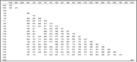
| 1 | 576 | 412 | 400 | 400 | 400 | 457 | 400 | 472 |
| 1000 | 427 | 400 | 400 | 400 | 400 | 466 | 425 | 425 |
| 1500 | 771 | 496 | 499 | 400 | 416 | 572 | 500 | 414 |
| 1600 | 889 | 548 | 552 | 400 | 438 | 576 | 520 | 422 |
| 1700 | 997 | 606 | 610 | 476 | 527 | 572 | 570 | 421 |
| 1820 | 1202 | 683 | 688 | 1202 | 691 | 577 | 669 | 420 |
| 1870 | 1960 | 937 | 993 | 2419 | 676 | 548 | 737 | 500 |
| 1913 | 3457 | 1695 | 1488 | 5233 | 1493 | 658 | 1387 | 637 |
| 1950 | 4578 | 2111 | 2841 | 9668 | 2503 | 639 | 1921 | 890 |
| 1973 | 11417 | 4988 | 6059 | 16179 | 4513 | 1225 | 11434 | 1410 |
| 2003 | 19912 | 6476 | 5397 | 28039 | 5786 | 3842 | 21218 | 1549 |
Switching to the GDP per capita measure indicates a different story that suggests that ACE complexity scores probably cannot necessarily be translated directly into GDP per capita terms. On the other hand, 1000 years have passed between 1000 BCE and 1 CE. In the West, the Greek city state complex had given way to the Roman Empire. In the East, Chinese fragmentation had been reversed by the rise of the Qin/Han Dynasties. In the year 1, accordingly, Western Europe and Asia are in the lead, Africa is third, and the other regions are rated as roughly equal. In 1000 CE, Asia retains its former lead, followed by Western Europe, Japan and Africa (all three with near-identical averages), with all other regions scoring at the 1 year minimum.
By 1500 CE, however, Maddison's data have Western Europe once more in the lead with Asia a distant second. The USSR, Japan, and Eastern Europe fall in the middle of the regional hierarchy. Latin America demonstrates some slight gain while Africa manifests steady decline. North America and Australia's position and wealth/technology level is shown as remaining unchanged for 1500 years. Then the scores change dramatically. The western European GDP per capita almost doubles by 1820. The Western Offshoots (North America and Australia / New Zealand) are not far behind. Eastern Europe, the USSR, and Latin America have made some progress with development levels that are about half those of the leaders. Average 1820 Asian and African GDP per capita are little changed from their 1500 levels. By the end of the 20th century, the Western Offshoots, Western Europe, and Japan have created strong leads. Latin America and the USSR are in the middle of the hierarchy but considerably behind the leaders. Eastern Europe, Asia, and Africa occupy the bottom of the regional hierarchy.
Table 5 reports the same data in regional rank order. The long-term outcome encompasses several significant shifts in relative standing. Western Europe is an early leader but falters in the Medieval Era before rising to the lead after the industrial revolution – a lead it does not maintain beyond the 19th century. The Western Offshoots remain in the technology/growth cellar throughout most of the ten millennia period studied before seizing the lead in the last century. Asia begins in the middle, rises to the lead in the first millennium CE, and then falls back toward the bottom. Japan's position oscillates – initially middle, then falling back to low, then to high, back to the middle, and then back to high. Eastern Europe and the USSR begin relatively high and decline to the middle. Latin America starts low and never exceeds a middle ranking. Africa tends to stay near the bottom except in the first millennium CE.
Scanning rank orders is one thing. We can improve on this form of data inspection by calculating Spearman Rank Order coefficients from observation to observation, as is done in Tables 6 and 7. Table 6 reports significant coefficients without any modification of the rank orders. Table 7 corrects for the more recent European migrations, following a technique utilized by Comin et al. (2010).[32] In Table 6, there are basically four clusters of coefficients.
Table 5. Regional rank orders
| Date | Western Europe | Eastern Europe | Former USSR | Western Offshoots | Latin America | Asia | Japan | Africa |
| 8000 | 2 | 1 | 4 | 8 | 7 | 3 | 5 | 6 |
| 4000 | 1 | 1 | 1 | 8 | 7 | 4 | 5 | 6 |
| 3000 | 1 | 1 | 1 | 8 | 5 | 4 | 6 | 7 |
| 2000 | 1 | 1 | 1 | 8 | 5 | 4 | 6 | 7 |
| 1000 | 1 | 1 | 1 | 7 | 5 | 6 | 7 | 4 |
| 1 | 1 | 4 | 5 | 5 | 5 | 3 | 5 | 2 |
| 1000 | 2 | 4 | 4 | 4 | 4 | 1 | 3 | 3 |
| 1500 | 1 | 5 | 4 | 8 | 6 | 2 | 3 | 7 |
| 1600 | 1 | 4 | 3 | 8 | 6 | 2 | 5 | 7 |
| 1700 | 1 | 3 | 2 | 7 | 6 | 4 | 5 | 8 |
| 1820 | 1 | 5 | 4 | 1 | 3 | 7 | 6 | 8 |
| 1870 | 2 | 4 | 3 | 1 | 6 | 7 | 5 | 8 |
| 1913 | 2 | 3 | 5 | 1 | 4 | 7 | 6 | 8 |
| 1950 | 2 | 5 | 3 | 1 | 4 | 8 | 6 | 7 |
| 1973 | 3 | 5 | 4 | 1 | 6 | 8 | 2 | 7 |
| 2003 | 3 | 4 | 6 | 1 | 5 | 7 | 2 | 8 |
Table 6. Significant Spearman rank order coefficients (only entries with P < 0.05 are shown; column numbers correspond to row numbers)
| Date | 1 | 2 | 3 | 4 | – | 8 | 9 | – | 11 | 12 | 13 | 14 | 15 | |
| 8000 | 1 |
|
|
|
|
|
|
|
|
|
|
|
|
|
| 4000 | 2 | .93 |
|
|
|
|
|
|
|
|
|
|
|
|
| 3000 | 3 | .85 | .93 |
|
|
|
|
|
|
|
|
|
|
|
| 2000 | 4 | .85 | .93 | 1.0 |
|
|
|
|
|
|
|
|
|
|
| 1000 | 5 |
| .77 | .81 | .81 |
|
|
|
|
|
|
|
|
|
| 1 | 6 |
|
|
|
|
|
|
|
|
|
|
|
|
|
| 1000 | 7 |
|
|
|
|
|
|
|
|
|
|
|
|
|
| 1500 | 8 |
| .71 |
|
|
|
|
|
|
|
|
|
|
|
| 1600 | 9 |
| .85 | .85 | .85 |
| .93 |
|
|
|
|
|
|
|
| 1700 | 10 |
| .90 | .93 | .93 |
| .79 | .91 |
|
|
|
|
|
|
| 1820 | 11 |
|
|
|
|
|
|
|
|
|
|
|
|
|
| 1870 | 12 |
|
|
|
|
|
|
|
| .85 |
|
|
|
|
| 1913 | 13 |
|
|
|
|
|
|
|
| .92 | .88 |
|
|
|
| 1950 | 14 |
|
|
|
|
|
|
|
| .95 | .91 | .88 |
|
|
| 1973 | 15 |
|
|
|
|
|
|
|
|
| .83 |
| .74 |
|
| 2003 | 16 |
|
|
|
|
|
|
|
|
| .76 | .76 |
| .91 |
The first cluster encompasses coefficients in the BCE era and indicates that the rank orders were similar between 8000 and 1000 BCE.[33] A second cluster suggests significant similarity in the rank orders between 4000 to 2000 BCE and 1500–1700 CE. The third cluster indicates little change in the rank orders between 1500 and 1700 CE. Finally, the fourth cluster singles out the period between 1820 and 2003 CE as roughly similar in terms of rankings.
If we control for the well-known impact of the early modern and modern European migrations, not too much changes. Table 7 still shows an early cluster in the BCE era and the second cluster of similarity linking the BCE era to the second period spanning from 1600 to 1913.[34] The third cluster, focusing on 1500–1700 CE in Table 4, disappears in Table 7. The modern fourth cluster, however, remains evident.
Table 7. Significant Spearman rank order coefficients adjusted for migration (only entries with P < 0.05 are shown; column numbers correspond to row numbers)
| Date | 1 | 2 | 3 | 4 | 5 | 6 | – | – | 11 | 12 | 13 | 14 | 15 | |
| 8000 | 1 |
|
|
|
|
|
|
|
|
|
|
|
|
|
| 4000 | 2 | .74 |
|
|
|
|
|
|
|
|
|
|
|
|
| 3000 | 3 | .83 | .86 |
|
|
|
|
|
|
|
|
|
|
|
| 2000 | 4 | .76 |
| .93 |
|
|
|
|
|
|
|
|
|
|
| 1000 | 5 |
|
| .81 | .93 |
|
|
|
|
|
|
|
|
|
| 1 | 6 |
|
|
|
|
|
|
|
|
|
|
|
|
|
| 1000 | 7 |
|
|
|
|
|
|
|
|
|
|
|
|
|
| 1500 | 8 |
|
|
|
|
| .74 |
|
|
|
|
|
|
|
| 1600 | 9 |
| .91 | .74 | .85 |
|
|
|
|
|
|
|
|
|
| 1700 | 10 |
| .88 | .88 | .76 |
|
|
|
|
|
|
|
|
|
| 1820 | 11 |
|
|
| .73 |
|
|
|
|
|
|
|
|
|
| 1870 | 12 |
|
|
| .76 |
|
|
|
| .85 |
|
|
|
|
| 1913 | 13 |
|
|
| .76 | .71 |
|
|
| .92 | .88 |
|
|
|
| 1950 | 14 |
|
|
|
|
|
|
|
| .95 | .91 | .88 |
|
|
| 1973 | 15 |
|
|
|
|
|
|
|
|
| .83 |
| .74 |
|
| 2003 | 16 |
|
|
|
|
|
|
|
|
| .76 | .76 |
| .91 |
Whatever these data represent, they do not support an argument for unmitigated technological and economic wealth persistence. To put it another way, it is rather hard to argue that in general national wealth was determined in 8000 BCE. The unadjusted regional rank order correlation in that year is –.143 (with the migration adjustment, the correlation is still only .286. The first-ranked region in 8000 BCE has slipped to number three ten thousand years later. The lowest-ranked region has climbed to number one. One thousand BCE is no more determinative (the unadjusted spearman coefficient is –.356 and .214 with an adjustment for migration). As in 8000 BCE, the two lowest ranking regions in 1000 BCE were in the lead by 2003. Africa, in the middle in 1000 BCE, has been at the bottom of the hierarchy for the past 500 years. Eastern Europe and the USSR, once among the ACE leaders, have struggled to stay in the middle of the rankings. Only the Asian and Latin American positions in 2003 closely resemble their 1000 BCE rankings.
What if we shift our focus to the year 1? The ability to predict from 1 to 2003 is about the same as when we use 8000 or 1000 BCE. The Spearman coefficient is –.380 if unadjusted and .262 if corrected for migration. Western Europe, Eastern Europe, the USSR, and Latin America have similar rankings at the end of the 20th century that they held in the year 1. Asia, Japan, Africa, and the Western Offshoots do not. Shifting to a predictive base in 1500 yields a better outcome. Although the unadjusted rank order coefficient is –.238, the adjusted correlation is .619. All but Asia and the Western Offshoots have similar rankings in 2003 that they held in 1500. What is missed, however, is that the mis-predicted regions include the most populous (Asia) and the richest (Western Offshoots) groups. Focusing on rank orders also downplays the size of the gap between the leaders and followers in 1500 and 2003. In 1500, the West European lead represented about a 2:1 lead over the lowest average GDP per capita in Africa and the Western Offshoots (then, of course, far less western and more indigenous North American and Australian). In 2003, the Western Offshoots lead is 19 times as large as the lowest regional GDP per capita (Africa).
But Comin et al. (2010) also encountered problems in using 1000 BCE and 0 CE data to predict to the current period. What about earlier shorter predictive capability? Between 4000 BCE and 1000 BCE, as noted earlier, there are few changes in the regional complexity hierarchy. All of the positions are not identical but they are very close. Between 1000 BCE to 1 CE, five regions retain similar positions, while three (Eastern Europe and the USSR decline, Asia vaults to a leading position) change their respective rankings. In the transition from 1 CE to 1500 CE, there is again little change. Only Africa falls substantially in the rankings.
Thus, the Maddisonian regional rankings are fairly stable in what might be called the ‘short’ or intermediate long-term, if we permit what is considered short to become shorter over time since the observations are not equally spaced. With sixteen observations over ten millennia, the rankings tend not to change all that much when one moves three observations forward in time. Attempts to predict beyond three observations, especially very long forecasts, work less well. That would suggest that technology and wealth distributions persist to some extent, but not indefinitely. With the partial exception of Latin America, none of the regions examined occupies a roughly similar position across all sixteen observations. Nor does it preclude substantial deviations from the persistence expectation. Asia was once very high in the hierarchy and then very low. Conceivably, it might be very high again, as demonstrated in the case of Japan (and perhaps China sometime in the future). The western offshoots, once at the bottom of the hierarchy for a very long term, eventually took the lead. Even if the offshoots should lose that lead, they are likely to remain near the top of the hierarchy for some time to come. Granted, the western offshoots generated their remarkable shift in the growth hierarchy initially through a combination of technological borrowing and endowment, their subsequent growth was due in part to the development of new technologies. Technological persistence, according to the Maddisonian data, is not destiny.
But what if we put the debatable Maddisonian data aside and look only at the city size data which are grouped in more defensible aggregations and which represent something more than one analyst's best retrospective guesstimate. The correlation pattern that emerges in these data (see Table 8) is both different and more simple than the one generated by Maddisonian GDP per capita figures. Yet, substantively, it leads to similar conclusions.
Three clusters are prominent. The first cluster encompasses 3700 BCE to 2000 BCE and represents the most ancient Mesopotamian concentration of cities. A second cluster began to emerge half way through the first millennium BCE and persists through 1800 CE. We might call this cluster the Silk Road grouping of cities stretching from the Mediterranean through South Asia to East Asia. The names and precise locations of the cities in each region that are most prominent in any given year vary but the regions retain their relative standings more or less, as demonstrated in Fig. 2.
The third cluster has a short life span (1900 and 1950). It represents the ascendance of the West and the technological leadership of Britain (London, Birmingham, Glasgow) and the United States (New York, Boston, Chicago, Detroit, Philadelphia, and Los Angeles). However, even by 1950, the large third world cities such as Calcutta and Bombay are also entering the top twenty-five cities in the world.
So, Table 8 demonstrates persistence as well. The first cluster predominated for 2000 years and then disintegrated, largely due to an inability to feed its expanded population with declining grain productivity. The second cluster of cities stretching from the Mediterranean to East Asia persisted for another 2000 years as the central armature of the world economy but was eventually overtaken by technological changes that had first traveled the Silk Roads but became concentrated in northwestern Europe and North America.
Table 8. City size correlations across time
Note: Only entries with P < 0.05 are shown. Pairwise, year-to-year, correlation coefficients are obtained based on the analysis of each region's share of city population. Years BCE in italics.
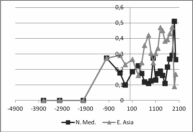
Fig. 2. Northern Mediterranean / West European and East Asian regional city share scores
The third cluster seems unlikely to retain its prominence for another 2000 years. If nothing else, city size is no longer a reliable instrument for capturing wealth and technological leadership as it once was. But the diffusion of wealth and technology is taking place faster than it once did (Comin and Hobijn 2010). The persistence of relative regional standings, as a consequence, must also be expected to change to varying extents as some once low ranking areas rise in the rankings. Yet there is also no reason to assume that all low-ranking regions will rise equally. In that respect, some mixture of persistence and change should be anticipated.
Since the patterns that emerge vary by indicator, do we need to pick and choose which one seems to have the greatest validity? The city size data demonstrate what we earlier described as largely missing from the earlier analyses of Olsson and Hibbs (2005) and Comin, Easterly, and Gong (2010). The city data isolate the Sumerian starting point for relatively large cities and underscore the ‘dumb-bell’ interaction between the Mediterranean and East Asia across Diamond's east-west axis. They also capture the post-1800 shift in cities due to industrialization. In these respects, the city size data most clearly conform to our understanding of the major shifts in, and evolution of, world history. Yet as long as all our indicators underline the limitations of persistence, there is really no reason to focus on one index alone. Multiple indicators show roughly similar mixtures of persistence and abrupt change.
Conclusion
Our point throughout has been that there are important limitations on path dependencies in historical economic growth patterns. Diamond's argument about east-west axis and the number of plants and large mammals certainly helps explain Eurasia's advantages over Africa and the Americas. It does not tell us too much about what happened within Eurasia after the creation of the world's continents. Whether we use biogeographical, societal complexity, GDP per capita, or city size indicators, there are very clear limits on the ability to predict in the long term who will be ahead in one year. Some places have been advantaged over others but not to the extent of predetermining economic growth well into the future. We cannot predict who precisely within Eurasia will get ahead based on Eurasia's initial advantage. Nor could we have predicted how long any Eurasian advantage might persist, except to say that it did not last forever. Using our indicators, we cannot predict who will be on ‘first base’ in 1 CE based on information in 1000 BCE. We cannot predict who will be ahead in 1950 or 1998 based on information in 1500. These prediction failures are not based on volatility in the data. There is substantial persistence across selected intervals. But there are also substantial shifts due ostensibly to leads and lags in technological leadership, demographic differentials, migration, climate change, disease, and warfare.
If we grant that human existence on planet Earth is characterized by some tendencies toward the stickiness of wealth and technological persistence subject to strong temporal limitations, the most interesting questions involve why these persistence tendencies fail to bar very substantial changes in regional and national rankings in economic wealth. We probably understand the reasons for technological and wealth persistence best. We do less well explaining how these characteristics are overwhelmed or in predicting how they may change in the future. It is conceivable, but by no means guaranteed, that an emphasis on very long-term shifts in technology and wealth will give us a better perspective on why the rich do not always get richer (or even stay rich) and why the poor sometimes improve their standings in the world pecking order.
References
Acemoglu D., and Johnson S. 2012. Why Nations Fail: The Origins of Power, Prosperity and Poverty. New York: Crown.
Acemoglu D., Johnson S., and Robinson J. A. 2001. The Colonial Origins of Comparative Development: An Empirical Investigation. American Economic Review 91: 1369–1401.
Acemoglu D., Johnson S., and Robinson J. A. 2002. Reversal of Fortune: Geography and Institutions in the Making of the Modern World Income Distribution. Quarterly Journal of Economics 117: 1231–1294.
Archer C. I., Ferris J. R., Herwig H. H., and Travers T. H. E. 2002. World History of Warfare. Lincoln, NE: University of Nebraska Press.
Bleaney M., and Dimico A. 2011. Biogeographical Conditions, the Transition to Agriculture, and Long-Run Growth. European Economic Review 55 (7): 943–954.
Burroughs W. J. 2005. Climate Change in Prehistory: The End of the Reign of Chaos. Cambridge: Cambridge University Press.
Chanda A., and Putterman L. 2005. State Effectiveness, Economic Growth, and the Age of States. States and Development: Historical Antecedents of Stagnation and Advance / Ed. by M. Lange, and D. Rueschemeyer, pp. 69–91. London: Palgrave Macmillan.
Chanda A., and Putterman L. 2007. Early States, Reversals and Catch-up in the Process of Economic Development. Scandinavian Journal of Economics 109: 387–413.
Chandler T. 1987. Four Thousand Years of Urban Growth: An Historical Census. Lewiston, NY – Queenston: St. David's University Press.
Chase-Dunn C., and Willard A. 1994. Cities in the Central Political-Military Network since CE 1200. Comparative Civilizations Review 30: 104–132.
Chase-Dunn C., Manning S., and Hall T. D. 2000. Rise and Fall: East-West Synchronicity and Indic Exceptionalism Reexamined. Social Science History 24(4): 721–748.
Chase-Dunn C., and Manning S. 2002. City Systems and World Systems: Four Millennia of City Growth and Decline. Cross-Cultural Research 36(4): 379–398.
Chase-Dunn C., Hall T., and Turchin P. 2007. World-Systems in the Biogeosphere: Urbanized State Formation, and Climate Change since the Iron Age. The World System and the Earth System: Global Socioenvironmental Change and Sustainability Since the Neolithic / Ed. by A. Hornbrog, and C. C. Crumley, pp. 132–148. Walnut Creek, CA: Left Coast Books.
Clark G. 2007. A Farewell to Alms: A Brief Economic History of the World. Princeton, NJ: Princeton University Press.
Comin D., Easterly W., and Gong E. 2010. Was the Wealth of Nations Determined in 1000 BC? American Economic Journal: Macroeconomics 2: 65–97.
Comin D., and Hobijn B. 2010. An Exploration of Technology Diffusion. American Economic Review 100: 2031–2059.
Diamond J. 1997. Guns, Germs and Steel: The Fate of Human Societies. New York: W.W. Norton.
Duijn J. J. van 1983. The Long Wave in Economic Life. London: George Allen and Unwin.
Findlay R., and O'Rourke K. H. 2007. Power and Plenty: Trade, War and the World Economy in the Second Millennium. Princeton, NJ: Princeton University Press.
Frachetti M. D., Spengler R. N., Fritz G. J., and Mar'yashev A. N. 2010. Earliest Direct Evidence for Broomcorn Millet and Wheat in the Central Eurasian Steppe Region. Antiquity 84: 993–1010.
Frank A. G. 1998. ReOrient: Global Economy in the Asian Age. Berkeley, CA: University of California Press.
Galor O. 2011. Unified Growth Theory. Princeton, NJ: Princeton University Press.
Hogg I., and Batchelor J. 1978. Naval Gun. Poole: Blandford Press.
Imamura K. 1996. Jomon and Yayoi: The Transition to Agriculture in Japanese Prehistory. The Origins and Spread of Agriculture and Pastoralism in Eurasia / Ed. by D. R. Harris, pp. 442–464. Washington: Smithsonian Institution Press.
Krieckhaus J. 2006. Dictating Development: How Europe Shaped the Global Periphery. Pittsburgh, PA: University of Pittsburgh Press.
Landes D. S. 1998. The Wealth and Poverty of Nations: Why Some Are So Rich and Some Are So Poor. New York: W.W. Norton.
Maddison A. 1995. Monitoring the World Economy, 1820–1992. Paris: OECD.
Maddison A. 2001. The World Economy: A Millennial Perspective. Paris: OECD.
Maddison A. 2007. Contours of the World Economy, 1–2030 AD: Essays in Macro-Economic History. Oxford: Oxford University Press.
Modelski G. 2003. World Cities: –3000 to 2000. Washington: Faros 2000.
Modelski G., and Thompson W. R. 1988. Sea Power in Global Politics, 1494–1993. London: Macmillan.
Modelski G., and Thompson W. R. 1996. Leading Sectors and World Powers: The Coevolution of Global Politics and Economics. Columbia, SC: University of South Carolina Press.
Morris I. 2010. Why the West Rules – For Now: The Patterns of History, and What They Reveal about the Future. New York: Farrar, Straus and Giroux.
Morris I. 2013. The Measure of Civilization: How Social Development Decides the Fate of Nations. Princeton, NJ: Princeton University Press.
Olsson O., and Hibbs D. A. Jr. 2005. Biogeography and Long-Run Economic Development. European Economic Review 49: 909–938.
Olsson O., and Paik C. 2013. A Western Reversal since the Neolithic? The Long-Run Impact of Early Agriculture. Working Papers in Economics 552, University of Gothenburg, Department of Economics. URL: https://gupea.ub.gu.se/bitstream/ 2077/32052/1/gupea_2077_32052.1.pdf.
Parker G. 1988. The Military Revolution: Military Innovation and the Rise of the West, 1500–1800. Cambridge: Cambridge University Press.
Parthasarathi P. 2011. Why Europe Grew Rich and Asia Did Not: Global Economic Divergence, 1600–1850. Cambridge: Cambridge University Press.
Peregrine P. N. 2003. Atlas of Cultural Evolution. World Cultures 14(1): 1–75.
Peregrine P. N., and Embers M. (Eds.) 2001. Encyclopedia of Prehistory. 9 vols. New York: Kluwer Academic/Plenum Publishers.
Pomeranz K. 2000. The Great Divergence: China, Europe and the Making of the Modern World Economy. Princeton, NJ: Princeton University Press.
Putterman L. 2008. Agriculture, Diffusion and Development: Ripple Effects of the Neolithic Revolution. Economica 75: 729–748.
Putterman L., and Weil D. 2009. Main Appendix to World Migration Matrix, 1500–2000, version 1.1. Brown University Department of Economics. URL: http://www. econ.brown.edu/fac/louis_putterman/world%20migration%20matrix.htm.
Putterman L., and Weil D. 2010. Post-1500 Population Flows and the Long Run Determinants of Economic Growth and Inequality. The Quarterly Journal of Economics 125(4): 1627–1682.
Rosenthal J.-L., and Wong R. B. 2011. Before and Beyond Divergence: The Politics of Economic Change in China and Europe. Cambridge, MA: Harvard University Press.
Sachs J., Mellinger A. D., and Gallup J. L. 2001. The Geography of Poverty and Wealth. Scientific American 284(3): 71–75.
Singer J. D., Bremer S., and Stuckey J. 2010 [1972]. Capability Distribution, Uncertainty, and Major Power War, 1820–1965. Peace, War, and Numbers / Ed. by B. Russett, pp. 19–48. Beverly Hills, CA: Sage.
Smith B. D. 1995. The Emergence of Agriculture. New York: Scientific American Library.
Thomas J. 1996. The Cultural Context of the First Use of Domesticates in Continental Central and Northwest Europe. The Origins and Spread of Agriculture and Pastoralism in Eurasia / Ed. by D. R. Harris, pp. 310–322. Washington: Smithsonian Institution Press.
Thompson W. R. 1999. The Military Superiority Thesis and the Ascendancy of Western Eurasia in the World System. Journal of World History 10: 143–178.
Turchin P., Adams J. M., and Hall T. D. 2006. East-West Orientation of Historical Empires and Modern States. Journal of World-Systems Research 12(2): 218–229.
Wong R. B. 1997. China Transformed: Historical Change and the Limits of European Experience. Ithaca, NY: Cornell University Press.
Validation Appendix
Any examination of behavior over multiple millennia is apt to rely on questionable assumptions and data. There are at least four possible threats to the validity of our results. One is that the Maddison data, especially for the earlier periods, are not very accurate. The problem, however, is that we lack alternative estimates of a similar nature to be able to assess Maddison's guesstimates about GDP per capita. Whether we will ever have alternative data, other than the city size data, encompassing the same period remains to be seen. In the interim, we have utilized what is available. Better estimates in the future would of course be very welcome. Similarly, using Maddison's older data forces us to use his regions as well. That is the way the data are made available. Would we like to experiment with different regional identifications? Certainly, but, again, we cannot at this time do so without abandon the GDP per capita scheme altogether.
However, there are two other debatable assumptions that we can assess. We use gross domestic product (GDP) per capita data to assess a question that is framed by Comin et al. as a matter of technological development. If we move away from indicators of technology per se, either in terms of societal complexity in the BCE era or GDP per capita in the CE era, have we modified substantially the argument at stake? We cannot do much more with the BCE era but there is a way to assess the relationship between GDP per capita and technological development in the more recent CE era. Less substantively perhaps, we also rely on rank orders to evaluate regional movement. Rank ordering in this case loses information by imposing an ordinal hierarchy on raw interval data. Why not just look at the raw interval data? The answer is that rank ordering simplifies the presentation of the findings. But it is worthwhile to check whether this simplification makes any meaningful difference to the analytical outcome.
We can make use of the Cross-Country Historical Adoption of Technology (CHAT) dataset developed by Comin and Hobijn (2010) and available at http://www.nber.org/data/chat. This data set focuses on the annual development of over 100 technologies in over 150 countries since 1800. We extracted a sample of some of the more important technologies of the past two centuries: steam ships, passenger trains, telegraph, telephone, electric power, cars, passenger planes, cellphones, and computers to create an overall technology score based on average, standardized scores on these nine technology foci. To preclude possible problems in interpreting the data, we also calculated scores based on the same data without technologies that had been introduced more than 100 years earlier. We also computed the relationship between overall technology scores and GDP per capita at the country and regional level, as shown in Table A1.[35]
The overall technology level is calculated in the following procedure. First, we take ‘raw’ technology indicators from the CHAT dataset which includes quantities such as the number of cars registered. We then normalized the raw values to population in order to obtain per capita indicators for the nine technology foci. Population data are taken from the National Material Capabilities dataset version 4 (Singer, Bremer and Stuckey 1972 [2010]). Second, the standardized score of each technology item k for country i is obtained as zik = (Xik – ![]() )/σk, where
)/σk, where ![]() is the mean value. Finally, overall technology level of country i is calculated by averaging Zik over all k's.
is the mean value. Finally, overall technology level of country i is calculated by averaging Zik over all k's.
Table A1. Technology-GDP per capita correlations
|
| Country-level |
| Regional-level |
|
|
| Original | Adjusted | Original | Adjusted |
| 1870 | 0.840 | 0.840 | 0.867* | 0.867* |
| 1913 | 0.850 | 0.850 | 0.954 | 0.954 |
| 1950 | 0.798 | 0.854 | 0.949 | 0.953 |
| 1973 | 0.760 | 0.778 | 0.940 | 0.884 |
| 1990 | 0.898 | 0.884 | 0.918 | 0.896 |
| 1998 | 0.910 | 0.915 | 0.991 | 0.994 |
Note: The adjustment involves removing technology that is older than 100 years from the calculation. Statistical significance is < 0.05 except for the two correlations with asterisks where p = <.10.
The outcome is that since 1870 at least, the general relationship between technological development and GDP per capita is quite high, especially at the regional level. It does not seem to matter if we control for old technology, the outcomes are quite similar. The possession of a high gross domestic product per capita indicates a high technological development score and vice versa. Of course, we do not find these relationships surprising in the contemporary period. The correlations do not test our assumption that a similar linkage between technological development and wealth holds over the long term but they do buttress our ability to make the assumption.
When we replace rank ordering with the raw scores suitably standardized, Table A2 summarizes the statistically significant correlations over time. The outcome looks much like the outcome reported in Table 6 using rank orders. There are some clusters of stability in the regional hierarchy, most notably demonstrated in the BCE era and in the post-1870 era. In between, there is not all that much correlation outside of the 1500–1700 CE period. It would appear that our finding that there are strong constraints on regional hierarchical stability in the really long term is not due to using rank ordered data. Similar outcomes emerge from the raw data as well.
Table A2. Regional hierarchy correlations over time with adjustment
| –8 0 0 0 | –4 0 0 0 | –3 0 0 0 | –2 0 0 0 | –1 0 0 0 | 1 | 1 0 0 0 | 1 5 0 0 | 1 6 0 0 | 1 7 0 0 | 1 8 0 0 | 1 8 2 0 | 1 8 7 0 | 1 9 1 3 | 1 9 5 0 | 1 9 7 3 | |
| –8000 |
|
|
|
|
|
|
|
|
|
|
|
|
|
|
|
|
| –4000 | .853 |
|
|
|
|
|
|
|
|
|
|
|
|
|
|
|
| –3000 | .888 | .903 |
|
|
|
|
|
|
|
|
|
|
|
|
|
|
| –2000 | .835 | .835 | .977 |
|
|
|
|
|
|
|
|
|
|
|
|
|
| –1000 | .695 | .636 | .849 | .941 |
|
|
|
|
|
|
|
|
|
|
|
|
| 1 |
|
|
|
|
|
|
|
|
|
|
|
|
|
|
|
|
| 1000 |
|
|
|
|
|
|
|
|
|
|
|
|
|
|
|
|
| 1500 | .743 |
|
|
|
| .815 |
|
| .989 |
|
|
|
|
|
|
|
| 1600 | .741 |
| .718 | .707 |
| .804 |
|
| .947 | .978 |
|
|
|
|
|
|
| 1700 |
|
|
|
|
| .744 |
|
|
|
|
|
|
|
|
|
|
| 1800 |
|
|
|
|
|
|
|
|
|
|
|
|
|
|
|
|
| 1820 |
|
|
|
|
|
|
|
|
|
|
|
|
|
|
|
|
| 1870 |
|
|
|
|
|
|
|
|
|
|
| .964 |
|
|
|
|
| 1913 |
|
|
|
|
|
|
|
|
|
|
| .941 | .984 |
|
|
|
| 1950 |
|
|
|
|
|
|
|
|
|
|
| .875 | .943 | .980 |
|
|
| 1973 |
|
|
|
|
|
|
|
|
|
|
| .845 | .847 | .873 | .851 |
|
| 2003 |
|
|
|
|
|
|
|
|
|
|
| .818 | .811 | .835 | .796 | .976 |
Note: Only correlations significant at the < .05 level are reported.
[1] In the past decade or so, Diamond (1997), Wong (1997), Frank (1998), Landes (1998), Pomeranz (2000), Maddison (2001), Clark (2007), Findlay and O'Rourke (2007), Morris (2010, 2013), Galor (2011), Parthasarathi (2011), Rosenthal and Wong (2011), among others, have appeared.
[2] The analyses of Chanda and Putterman (2005, 2007), Putterman (2008), and Bleaney and Dimico (2011) reinforce Olsson and Hibbs' finding that an earlier start on agriculture is beneficial to income levels much later.
[3] See Acemoglu and Johnson (2012: 51–56), among others, for a critique of the Diamond argument. Olsson and Paik (2012) develop and test a very interesting argument about the timing of agriculture that substantially modifies the idea of early biogeographical advantages. Basically, the idea is that the earliest adopters of agriculture tended also to adopt highly autocratic political systems which subsequently led to poor or poorer than might otherwise have been anticipated economic performance. Later adopters tended to develop different, less extractive, institutions and, therefore, enjoyed better economic development.
[4] See Turchin and Hall (2006) for an extension of the argument to imperial development.
[5] There is no question that Eurasia is the largest populated continent and that it encompasses more plants and large mammals that can be used for economic development purposes. Unlike the north-south alignment of Americas and Africa with major, mid-continental blockages to diffusion, it is not only possible for plants, animals, and technological innovations in one end of Eurasia to travel to the other; it is difficult to account for Eurasian development without tracking the diffusions. Parts of Eurasia certainly experienced earlier agricultural and industrial revolutions than elsewhere.
[6] At one point, Diamond (1997) suggests that any part of Eurasia might have seized the development lead but later suggests that western Eurasia was favored over eastern Eurasia.
[7] Actually, Olsson and Hibbs (2005) say that their initial observations are based on 11,000 BCE because it is around this time that unequal levels of development began to emerge due to population migrations that had started in Africa some 70,000 years earlier and climate change that melted glaciers thereby making agriculture possible in the northern hemisphere.
[8] Perhaps the main exceptions are the ‘out of Africa’ movements 50 to 100, 000 years ago in which our species colonized the world and Greek and Phoenician colonization in the first millennium BCE.
[9] See, for instance, the analyses reported in Acemoglu, Johnson, and Robinson (2001, 2002); Sachs, Mellinger, and Gallup (2001); and Krieckhaus (2006).
[10] In some of these cases, migrations of ‘barbarian’ tribes are part of the decline explanations. However, it is easier to argue that imperial decline or weaknesses attracted the migrations and that because of the decline, the migrations were more difficult to manage than it is to contend that migrations were either the or a principal cause of the decline. Yet many of the countless tribal migrations did not involve individuals with technological skills moving into low-tech environments. It was often the other way around although tribal warriors did sometimes possess superior weaponry technology – as illustrated by the Hyksos early second millennium BCE movement into Egypt with chariots and stronger bows. However, exceptions on the order of the Phoenician founding of Carthage certainly occurred.
[11] One of the Comin et al. (2010) technology indicators for 1500 is ships with 180+ guns. It seems highly unlikely that any ship in the world carried (or could carry without sinking) 180 guns or cannon as early as 1500. At this time, Portuguese ships were armed with artillery that more closely resembled mortars more than cannons but the naos were fairly small and only a few pieces of artillery could be carried on board ship. On the other hand, if the opposition possessed no maritime artillery, as in the Indian Ocean, a few guns often (but not always) sufficed. Henry VIII of England did have several very large ships constructed in the second decade of the 16th century and at least one (The Great Harry) carried 184 guns. But most of these guns were too small to do damage to ships and were used to repel boarders. The ships proved hard to sail, at least one capsized in part due to the heavy guns carried, and by the 1530s, the surviving ships were carrying fewer guns. See Hogg and Batchelor (1978: 11) and Archer et al. (2002: 262–263).
[12] ACE is based on the nine-volume Encyclopedia of Prehistory (Peregrine and Embers 2001).
[13] See, for instance, the list of innovations examined in van Duijn (1983: 178).
[14] While there is no reason to spend a great deal of time on a single indicator, the technological significance of cavalry, at least on or after 1500, is questionable. At one point, the adoption of cavalry and, later, the stirrup, reflected significant changes in military technology but in places that had access to horses these changes long preceded 1500 CE. Central Eurasian nomads led the way but did not necessarily create standing cavalries. Assyrians began to emulate their practices early in the first millennium BCE, as did the Chinese some 600 years later. After 1500, the maintenance of large cavalry units in Eurasia were more likely to signify aristocratic and agrarian constraints on technological development. Thus, as a 1500 CE indicator, it really only serves to differentiate places that had horses and those that did not (the Americas, the southern half of Africa, and Australia).
[15] Compare Parker (1988) and Thompson (1999) on this question.
[16] Switching from states to regions does not eliminate the center-periphery problem but there does seem to be some tendency for regions to become more homogenous over time in terms of existing levels of economic development.
[17] Maddison seems to have preferred to ignore the Middle East as much as possible in his data collection efforts. Presumably, that tendency reflects a desire to evade the problems associated with small, oil rich states and, perhaps, poor data for the poorer members of that region. To the extent that he dealt with this region, it is usually considered as a western extension of Asia. He classifies Egypt as an African state.
[18] That is to say that Maddison's older data are not available independent of his regional aggregations.
[19] Yet consider Comin et al.'s (2010).
[20] However, see as well the very strong correlations we find between regional GDP per capita and regional technological standings and report in the Appendix.
[21] On this subject, see Chase-Dunn and Willard (1994); Chase-Dunn, Manning, and Hall (2000); Chase-Dunn and Manning (2002); Modelski (2003); and Chase-Dunn, Hall and Turchin (2007).
[22] Choosing to look only at the top 25 is arbitrary but in older periods, cities tend to become fairly small as one moves beyond the first 25. Restricting our focus to the top 25 thus reduces some of the noise that might be introduced by casting the net farther down the size line. It also helps that Chandler (1987) provides more locational information for the first 25. However, Chandler identifies sources of imperial control whereas we are focused on geographical location.
[23] There are a small number of large cities that do not fit in any of these regions (for instance, a few cities rise to make the top twenty-five threshold in the Arabian Peninsula) but their relative prominence tends to be too short-lived to expand the number of regions.
[24] Only one city changes its regional location. We code Constantinople as Northern Mediterranean prior to the arrival of the Ottoman Turks and Southern Mediterranean thereafter.
[25] Another problem is that some regions have experienced climate changes over the last ten millennia. See, e.g., Burroughs (2005).
[26] A reviewer, contrary to Diamond, has argued that Africa has a long east-west axis stretching across the Sahel to the Horn. We do not find this axis very compelling because of the difficulties in crossing (we know French soldiers had problems making the crossing to set up the 1898 Fashoda crisis) and the limited historical traffic actually traversing it (at best, presumably, small groups of desert nomads). More important, large and urbanized population centers at both ends, which may be the most critical factor in differentiating between east-west and north-south interactions even though it goes beyond the Diamond argument, are missing in the African case. Eurasia's east-west axis was not all that easy to traverse but traders at least had strong profit incentives to make the effort. Just how important people were as carriers to the diffusion of seeds and animals across Eurasia is not entirely clear. Nonetheless, we will check our results to see how critical the presence or absence of an African east-west axis is to the outcome.
[27] We did not give equal weight to the continental axis and plants/mammals indicators because Eurasia already scores relatively highly on the distribution of domesticated flora and fauna. In some respects, the irony is that the super-region or continent that experienced the most diffusion needed it least. The exception to this observation is the much later diffusion of industrial technology from China to Europe in the first half of the second millennium CE. On this point, see, among a number of others, Modelski and Thompson (1996).
[28] In cases in which the timing is indicated as falling within a range of years, the middle point between the high and low timing dates is used for this calculation.
[29] Ideally, we might have weighted the averaging process by the size of the group but this information, unsurprisingly, is not available.
[30] Olsson and Paik's (2012) argument and findings, for example, suggest differentiating Southern from Northern Europe in terms of the timing of adopting agriculture and its implications.
[31] Space considerations preclude reporting the full correlation matrices. Thus, only significant correlations are shown. The full matrices are available from the authors on request.
[32] Comin et al. (2010) utilize Putterman and Weil's (2009) matrix on post-1500 migrations to correct 1500 and onward outcomes by the proportion of national population that has migrated into the country. We do the same for regional aggregations. Putterman and Weil's original migration matrix includes information of the migration from 1500 to 2000 for 165 countries. This state-level matrix was converted to a regional-level matrix, so that the modified matrix gives the proportions of each region's population in the year of 2000 that resided in its own and other regions in 1500. As in Comin et al., pre-1500 regional rankings were generated by pre-multiplying the ‘raw’ vectors of wealth/technology scores by the modified (regional) migration matrix. The resulting historical rankings thus reflect the post-1500 migration on the regional basis. For details of the migration matrix, see Putterman and Weil (2009, 2010).
[33] This first cluster is much diminished in terms of the number and size of the coefficients if Africa is coded as possessing an east-west axis.
[34] The first cluster almost disappears when provision is made for an east-west axis in Africa. The second and third clusters remain roughly the same.
[35] The 1870–1998 interval is dictated by the absence of much earlier and more recent information in CHAT. In addition, one has to be careful in using CHAT data because there are some problems with data listed in non-equivalent units that can be traced back directly to the sources that were utilized. We attempted to correct these problems prior to the analysis.