Global Fear and Long Range Political Cycles: A Mathematical Model

Author: Widdowson, Marc
Almanac: History & Mathematics:Historical and Technological Dynamics: Factors, Cycles, and Trends

The Polity IV Time Series of the Center for Systemic Peace can be used to classify world polities since 1800 into autocracies, democracies and ‘anocracies’ (between the two). The relative fractions of each type turn out to exhibit, to first order, simple mathematical regularities. These are explained by a mathematical model drawing on the anthropology of fear and its observation that political and economic insecurity predispose people to support authoritarian leadership, along with the established result that middling regimes present the greatest amounts of conflict and instability. The result is an oscillation between autocracy and anocracy, superimposed on which there is the spread of democracy through contagious learning. Awareness of this dynamic can help us understand how present-day conditions may shape world political evolution many decades ahead, as well as get early warning of whether democratisation really is locked in or may be reversed by future fear-inducing events.

Keywords: political evolution, democratisation, fear, insecurity.

Introduction

The Polity IV Time Series (INSCR 2017) provides an annual numerical classification of the type of polity possessed by each country included in the dataset, from 1800 to the present.

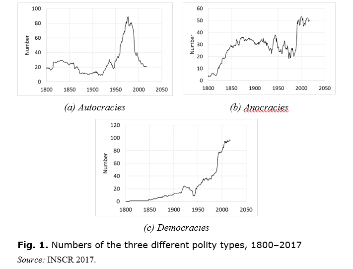
The ‘Polity Score’ captures [the] regime authority spectrum on a 21-point scale ranging from -10 (hereditary monarchy) to +10 (consolidated democracy). The Polity scores can also be converted into regime categories in a suggested three-part categorization of ‘autocracies’ (–10 to –6), ‘anocracies’ (–5 to +5 and three special values: –66, –77 and –88), and ‘democracies’ (+6 to +10) (Center for Systemic Peace n.d.).

‘Anocracies’ are defined as ‘mixed, or incoherent, authority regimes’ (Ibid.). These often have outward institutions of democracy but impose de facto restrictions on its practice, such as corrupt elections or intimidation and suppression of political opponents.

Fig. 1 shows the changing numbers of countries that were autocracies, anocracies and democracies from 1800 to 2017. Some qualitative features that might be noticed are: (a) the overall, seemingly accelerating growth of the number of democracies; (b) an increase in the number of autocracies from the 1920s to 1945, reflecting the rise of fascist regimes; and (c) a large spike in the number of autocracies post-1950, during the era of European decolonisation. In the latter respect, one could say that the democratic deficit of the developing world during the second half of the 20^th century was a transient phenomenon as these new countries shed the legacy of colonialism, and they are now treading the established path towards democracy, perhaps via anocracy.

Growth of Number of Polities

Fig. 2 plots the total number of countries included in the Polity IV dataset over time. It is apparent that this number has tended to increase.

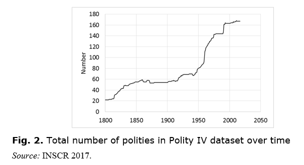
Does the increase in the number of polities exhibit any kind of regularity? One possibility is a straight line. Another is an exponential. A third is a logistic. We can also consider adding a constant to the exponential and logistic cases. The results of fitting these various curves to the data of Fig. 2 are shown in Table 1. The goodness of fit is measured by an adjusted R-squared value (hereafter referred to as R2) that takes into account the number of degrees of freedom (i.e. the number of free parameters to be determined).[1] This provides a fairer comparison between fitted models with different numbers of parameters, given that a higher number of parameters makes it easier to get a good fit.

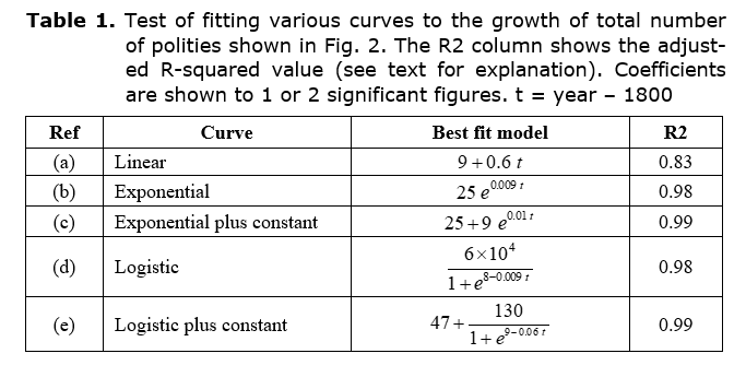
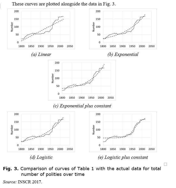
Table 1 and Fig. 3 show that there is little to choose between the exponential and logistic models, all of which explain much more of the variation in the data (i.e. have a higher R2) than does the linear model. In fact, the logistic model without a constant is essentially the same as the exponential model without a constant, given that the upper limit (6 ´ 10⁴) is much larger than the current number of polities (167) so we really only see the initial exponential-like part of the logistic curve. If we assume that a constant is added to the logistic curve, we can get a closer fit at the top end, with the characteristic turnover and plateauing of a logistic curve. However, this is at the expense of a worse fit at the bottom end. It is not clear that the downturn at the top end is really the result of saturation of a logistic growth process or whether it is a second order deviation from the primary trend, like those lower down the curve. Overall, the logistic model plus constant is not particularly convincing unless we (illegitimately) ignore the part of the dataset that does not fit.

The upshot of this is that we should probably regard the growth of the total number of polities over the period in question (1800–2017) as an exponential process. Before 1800, it may have been constant or followed some other trajectory, and in the future it may reach saturation and be revealed as actually logistic. However, for the data in view, it is exponential. If  represents the total number of polities, the growth process obeys the equation (using the dot-notation to represent a time derivative)

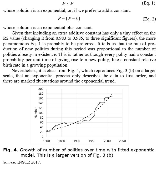
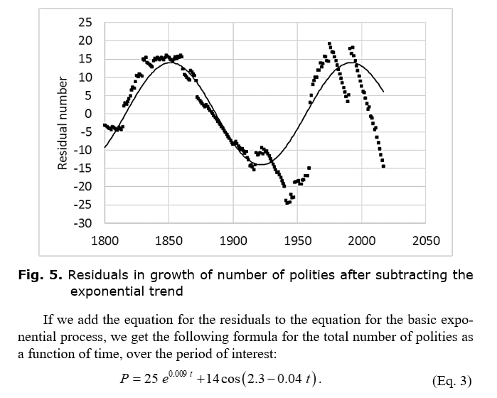
In Fig. 5, we plot the residuals after subtracting the exponential trend from the raw data. There is a hint that this may follow something close to a sinusoidal oscillation. Indeed, the residuals can be described by the Eq. 14 cos(2.3 – 0.04t) where t = year – 1800, as before. This equation is also plotted in Fig. 5, as the solid line. The R2 value is 0.66.

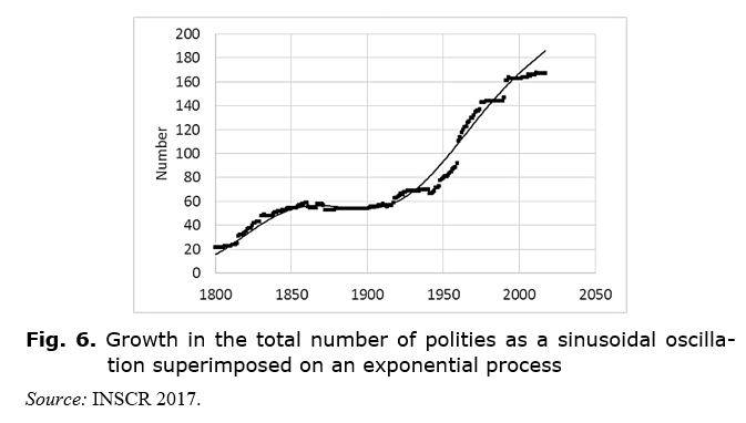
This is plotted in Fig. 6. The deviations from the exponential process thus appear not to have been completely random but were characterised largely by some oscillatory mechanism. Such a sinusoidal oscillation occurs when deviations from trend have inertia, i.e. tend to keep increasing / decreasing at the rate they are already increasing / decreasing, but are opposed by a restoring force whose strength is proportional to the size of the deviation. In symbols, , where  is the size of the deviation (the number of polities above or below the expected exponential trend). In other words, if new polities were being created ‘too slowly’, the rate would not only speed up towards the expected exponential growth but would shoot beyond it, where it would slow down then move back towards the trend and again overshoot on the negative side. This created a roughly regular oscillation around the trend.

Putting these together, we therefore have a dynamic in which (a) polities tended to stimulate the emergence of other polities, so that the more polities in existence the faster new ones would be created, and (b) the rate of increase of polities would speed up if it were slower than expected for the given number of existing polities, and slow down if it were faster, so that it did not converge on the expected baseline growth rate but swung either side of it. To put the latter point another way, the process of creating new polities exhibited lag, so that it took a while to respond to opportunity and then took a while to slow down again after it had begun to run away with itself.

A number of alternative possible forms have been tried for the oscillatory residual term, all more complicated than the simple sine wave incorporated in Eq. (3) and all involving some kind of changing amplitude to the sine wave. Although it is possible to get higher R2 values in this way, particularly with superposed oscillations producing a beat (an oscillation whose amplitude oscillates), the gain in quantitative agreement, traded off against increased complexity, does not seem to be justified by improved theoretical insight, at least not so far.

Changes in the Relative Proportions
of Different Polity Types

To investigate changes not just in the number of polities but in their types, it will be helpful to focus on relative proportions. They are plotted in Fig. 7. Thus, if ,  and represent the absolute numbers of autocracies, anocracies and democracies, respectively, then Fig. 1 above shows the variation in ,  and D, while Fig. 7 shows the variation in their fractions, ,  and , where ,  and . 

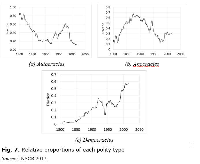
We again see an overall rise in the democracy curve, so that there were not just more democracies in absolute terms but the fraction of polities that were democracies also increased with time, from zero at the start of the period to over 50 % by 2017. In the case of anocracies, one can see something that looks possibly like a sinusoidal oscillation, and the same is true for autocracies, though the amplitude of the second autocracy peak is lower than that of the first. Since we have factored out the absolute variation in the number of polities, normalising the total number to 1 throughout and focusing only on relative proportions, these oscillations in autocracy and anocracy are not the same as the oscillation in total number found above (see Eq. 3, Fig. 5, 6). They are independent phenomena, though it is possible that there is some link between them.

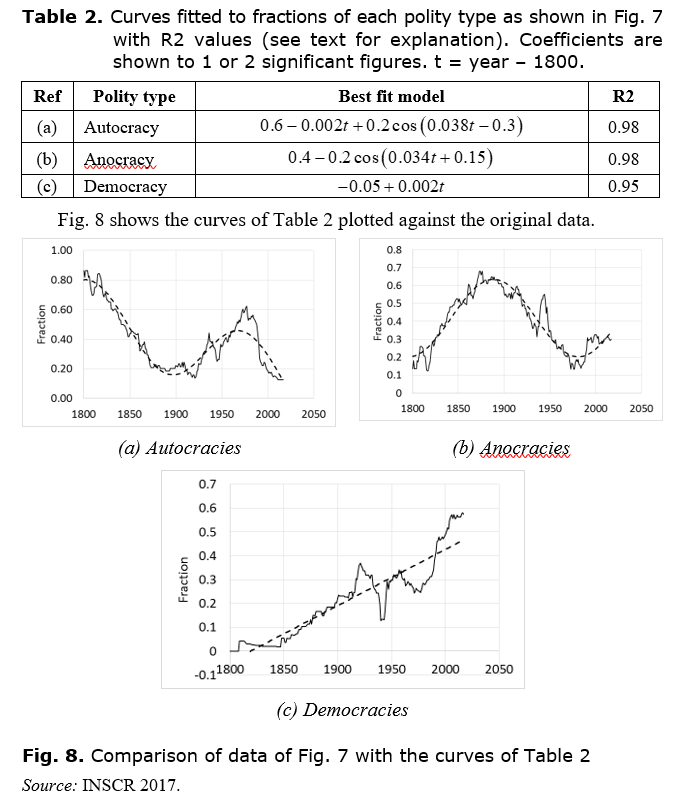
The next step is to find best fit equations for each of the autocracy, anocracy and democracy curves. They are shown in Table 2. A number of forms were tried in each case, and those in the table represent a trade-off between simplicity and quality of fit. For autocracy, we find a sinusoidal oscillation 0.2 cos(0.038t – 0.3) around a downward sloping line (0.6 – 0.002t). For anocracy, we find a sinusoidal oscillation 0.2 cos(0.034t + 0.15) around a constant value (0.4). For democracy, we find an ascending straight line (–0.05 + 0.002t).

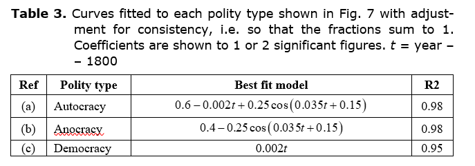
Strictly we require that the fractions of autocracy, anocracy and democracy should sum to 1. However, the equations of Table 2, which were obtained by just finding the best fit to each curve considered on its own, do not do so exactly. For example, the fact that the autocracy and anocracy oscillations have different frequencies means that they will move slowly in and out of phase, and their sum will oscillate. Nevertheless, one can make some small adjustments to the coefficients of the best fit equations that ensure the fractions do sum to 1. This is a manual operation of trial and error. One possible solution is shown in Table 3, which should be considered ‘close enough’ rather than necessarily ideal in a statistical sense. The main changes are to drop the constant term for democracy, and to make the autocracy and anocracy fluctuations of the same frequency and in anti-phase so that they exactly cancel. This adjustment does not noticeably worsen the fit (R2) to the degree of significance shown. It can be checked, just by adding the three equations together, that the terms in  cancel each other, leaving just the constant terms, which add to .

The relative dynamics of the three polity types are illustrated in Fig. 9. We can conceptualise this as follows. Polities oscillate in and out of anocracy. Among the non-anocracies, the democracy share increases steadily as though those gains are permanent and ‘locked in’– once polities have become democratic they remain so. Autocracies are squeezed between the two – not only does their share fluctuate as the share of anocracies rises and falls but their share is also steadily eroded by the growth of democracy.

While this provides an intuitive picture of the dynamics of Table 3, we need to be clear that Fig. 9 represents the fractions of polities of the different types, not actual polities. This means, for example that, since the total number of polities is increasing exponentially, the number of democracies is increasing faster than the linear rise in the fraction. Similarly, the fluctuation in anocracy does not necessarily mean that individual polities change type; it could also be caused by fluctuation in the tendency of new polities to emerge as anocracies or non-anocracies. Thus, the dynamics of actual polities are more complex than those of the shares of different types.

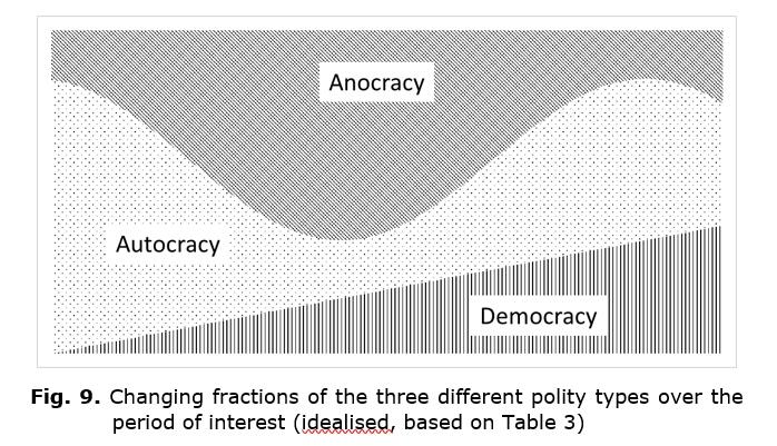
It is clear that the dynamics of Fig. 9 cannot go on forever. Soon the democracy share will begin to interfere with the autocracy-anocracy oscillation, and eventually the democracy share will reach 1, after which it will have to stop increasing. Thus, Fig. 9 describes the dynamics over the historical two centuries covered by the Polity IV database, whereas distortions to these dynamics should now be beginning to emerge.

Focus on Democracy

For Modelski and Perry (1991, 2002), the global spread of democracy is a learning process, so that the share of democracies among world polities might be expected to follow a logistic curve. Over the period in question, it is only the relatively straight central portion of the curve that is visible. Modelski and Perry estimate that the 90 % saturation point, when the turnover of the curve becomes unmistakable, will be reached in the early 22^nd century.

In Table 3, the linear model for democracy has the lowest R2 value at 0.95. An alternative would be an exponential model, given that the early part of a logistic curve is exponential. This turns out to have the best fit form of  and an identical R2 of 0.95 to two significant figures. The linear and exponential models are compared in Fig. 10. It can be seen that, while the exponential model perhaps fits better at the upper end, the linear model seems to reflect better the overall trend, and so will be preferred here. That is to say, the assumption of linearity is adequate for present purposes, even though, in long term perspective, it must deviate from linearity and is very probably logistic.

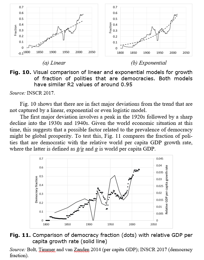
The study of Fig. 11 reveals a suggestive synchrony between the prevalence of democracy and the growth of prosperity. Of course, this does not prove causality. The fluctuations in prosperity sometimes come before the fluctuations in democracy, and sometimes come afterwards, which speaks against there being a causal link. On the other hand, the GDP per capita data are coarse-grained, at intervals of a decade or more, so that the lags and leads in peaks and troughs lie within the margin of error. Furthermore, even if causality is accepted, this does not prove in which direction it operates. It might be that economic downturns produce a deterioration in democratic institutions, or it might be the other way around, that a lack of democracy inhibits free enterprise and leads to economic decline.

There are nevertheless reasons for supposing that economic hardship will be associated with a turning away from democracy. According to the anthropology of fear, the experience of political and economic insecurity causes people to adopt more extreme attitudes and to be more willing to support authoritarian leaders. In Northern Ireland, sectarian conflict meant that those who were ready to reach accommodation with the other side kept quiet, so as not to appear disloyal to their communities, and intransigence became the dominant value (McCartney 1991). People who feel a lack of control over their lives become suspicious of others and they put their trust in figures perceived as powerful and as offering tangible solutions – not just material solutions but also ideological solutions, such as nationalism, restoring self-respect (Merolla and Zechmeister 2009: 9; Smallman 2002: 186–187). Such insecure populations are characterised by ‘obedience to authority, moral absolutism and conformity, intolerance and punitiveness toward dissidents and deviants, animosity and aggression against racial and ethnic out groups’ (Merolla and Zechmeister 2009: 30; see also Pozrvanović 1993). These values are reinforced by peer pressure and by observation of violence or injustice (Corradi 1992; Muldoon 2003: 162). Thus, societal coping mechanisms for dealing with fear, including fear induced by economic insecurity, tend to threaten the fabric of democracy and make autocracy a viable, indeed attractive, alternative.

Fig. 12 compares the fraction of polities that are democracies with the GDP per capita growth rate (NB ġ, not ġ/g as in Fig. 11).

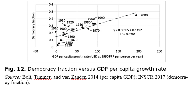
The chart of Fig. 12 shows some correlation between economic growth and growth of democracy. The correlation is not solely due to the two quantities being independently correlated with time (i.e. just both happening to grow over time without any link between them) because both per capita GDP growth and democracy fraction sometimes fell backwards to approximately the same extent, maintaining the roughly linear relationship. On the other hand, if fear is the key factor, we would not expect the correlation to be perfect since there are other influences on fear and insecurity besides the strength or weakness of economic growth.

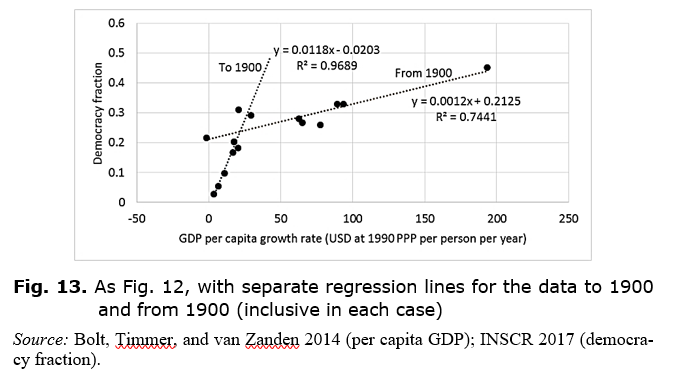
Fig. 12 also demonstrates that there may have been a shift in the relationship between the quantities around the turn of the 20^th century. This is explored in Fig. 13, which performs separate linear estimations for the data to 1900 and from 1900. It appears that, after 1900, democratisation became less sensitive to changes in prosperity, perhaps due to the revolution in communications shifting emphasis to other processes affecting its spread. This possibility and the role of other factors influencing fear is left for future work.

Changes in Absolute Numbers

Returning to the absolute numbers of each type of polity, one can model these as the product of the total number of polities and the fraction of each type of polity. That is, in Eq. (3) we have a formula for P(t), the total number of polities, and in Table 3 we have formulas for а(t), n(t) and d(t), the fractions of autocracies, anocracies and democracies respectively, so we can obtain formulas for А(t), N(t) and D(t), the numbers of autocracies, anocracies and democracies, by

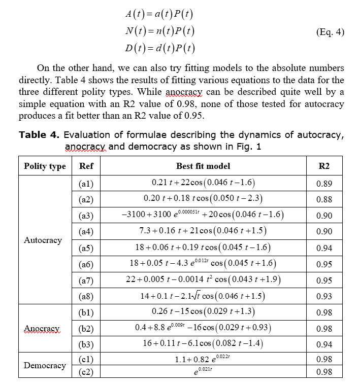
For each polity type, the equations that best combine simplicity with a high R2 value are as shown in Table 5. Remarkably, democracy is well described by a simple exponential with just one parameter. The value of the parameter, shown as 0.021 in Table 5, is more precisely 0.0214168. A slightly better fit can be obtained with  but this hardly affects the R2 value (0.980933 versus 0.980931). Anocracy is described by a sinusoidal oscillation plus a term that grows linearly with time. Autocracy is described by a sinusoidal oscillation whose amplitude grows with the square of time, plus a constant and a term that grows linearly with time.

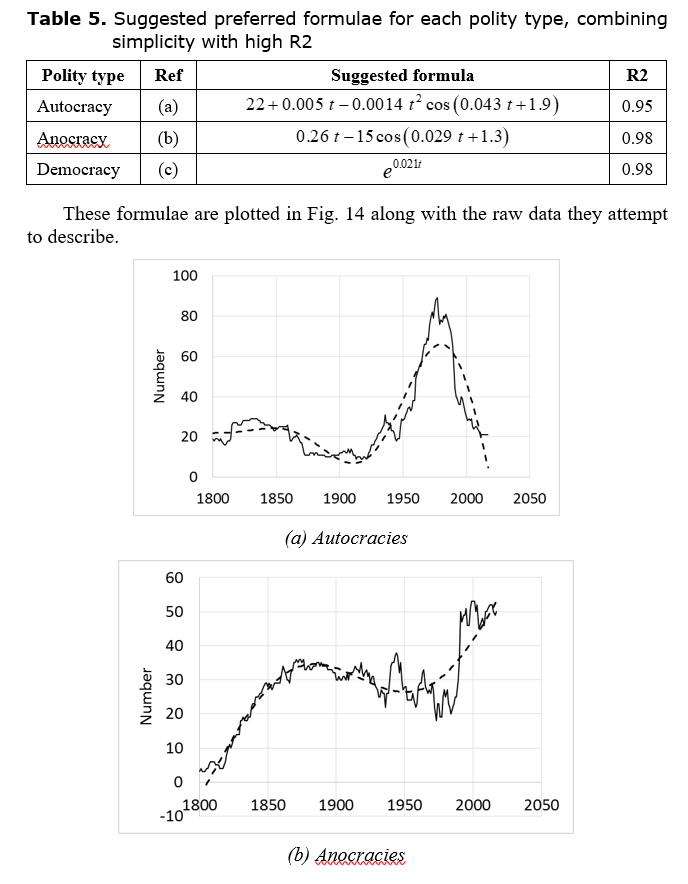
Fig. 14. Comparison of formulae of Table 5 with the original data

Source: INSCR 2017.

It can be seen that while the formula for democracies seems to capture a genuine feature of the dynamics and that for anocracies does so to some extent, though perhaps less convincingly, that for autocracies looks rather forced. In the case of autocracies, it proves difficult to obtain a formula that follows the initial up-down motion as well as rising and falling fast enough for the second peak. This second peak reflects the surge in autocracies following European decolonisation. It therefore seems that this process of decolonisation and its effects had rather unique features, requiring a more complex representation than those tested in Table 4, possibly requiring additional variables and not being a straightforward function of time. This is left for future exploration.

A final point worth considering is the phase relationship between the two oscillating polity types, namely autocracies and anocracies. In the case of the autocracy and anocracy fractions, as shown in Table 3, the oscillations are in antiphase, i.e. 180° or π radians out of phase. This is necessary in order for them to cancel, so that the total of all three polity types can sum to 1. However, when we consider absolute numbers, there is no such requirement, since the total number of polities is not fixed. It is possible for the numbers of autocracies and anocracies to have some other phase relationship so that their combined sum fluctuates.

According to Table 5, the autocracy and anocracy oscillations actually have different frequencies, of 0.043 and 0.029, which means they do not have a fixed phase relationship. However, as Fig. 14 (a) suggests, the frequency for autocracies may be too high since it creates too short a distance between the first and second peaks (even if it optimises the fit overall). There is also some leeway in the frequency for anocracies, since the bottom of the trough around 1950 to 2000 is poorly defined. Consequently, we can adjust the two frequencies to be the same and still obtain, at least visually, a reasonable fit with regard to the placing of peaks and troughs (see Fig. 15). This superimposes two sinusoidal oscillations on the raw data, ignoring amplitude changes but lining up peaks and troughs. The compromise frequency of the oscillations is chosen
as 0.04.

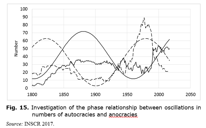
When we match the autocracy and anocracy oscillations to same-frequency but different-phase sine waves, as in Fig. 15, we find that they are 135° or 3π/4 radians out of phase. We would thus expect their sum to fluctuate. This fluctuation will have the same frequency as the underlying oscillation, i.e. 0.04, assuming the frequency shown in Fig. 15. Indeed this is the frequency we found for the oscillation in the growth of the number of polities (see Eq. 3).

If autocracies and anocracies were 90° or π/2 radians out of phase, they would effectively correspond to sine and cosine respectively (because sine and cosine are 90° = π/2 radians out of phase). Since the derivative of sine is cosine and the derivative of cosine is negative sine, this would mean that autocracies and anocracies would be related by  and , which says that anocracies cause autocracies to increase in number and autocracies cause anocracies to decrease in number, potentially providing a simple explanation for their tendency to oscillate (i.e. as anocracies increase in number they would cause autocracies to increase, which would cause anocracies to decrease again).

However, autocracies and anocracies are not 90° out of phase but 135° out of phase, and therefore the relations  and  do not apply. This tells us that the autocracy-anocracy oscillation is not due to a direct interaction between the numbers of autocracies and anocracies and must involve the intervention of some other variable. We will introduce such a variable in the mathematical model developed below.

Emergence and Transformation of Polities

Two suggestions made above were that democracies tend to spread by a learning process, and that changes in the number of autocracies may be related to the prevalence of fear or political and economic insecurity. We will investigate these propositions by considering some quantitative aspects of the formation and transformation of polities.

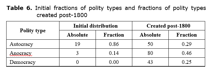
Table 6 shows the initial distribution of polity types in 1800, at the start of the Polity IV dataset, and the distribution of polity types created post-1800. It can be seen that, at the beginning of the period, the vast majority of polities were autocracies, and none were democracies. However, over the course of the period, nearly half of new polities emerged as anocracies, while the others were split almost equally between autocracies and democracies.

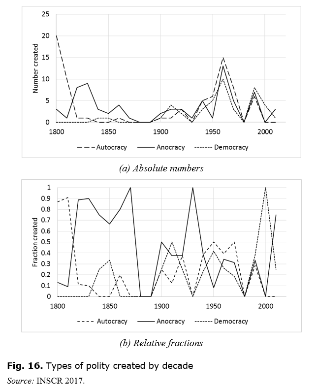
For polities created, we can break the figures down by decade as shown in Fig. 16 (a) (absolute numbers) and (b) (relative fractions). We see from this that the creation of democracies occurred in a series of pulses, around 1840, 1910, 1960 and 1990. Each of these pulses also involved the creation of other polity types, and there has been no clear trend in any particular direction. That is, we cannot say that there is any overall tendency for newly created polities to be of one dominant type, nor can we say that a dominant type is emerging.

Although the learning effect of democratisation is not clearly evident in the creation of polities, we can test for this effect in another way by examining whether democracies were more likely to arise from democracies. Thus, many of the newly created polities were formed by gaining independence from colonial empires or by the break-up of existing polities. We will investigate whether the type of the source polity affected the type of the newly created polity. To do this, the polities listed in the Polity IV database as coming into existence post-1800 were each examined and, if the polity was created by some sort of fission from an already existing polity, the type of that polity was noted. If the polity was not created from an existing polity, its source polity was noted as N/A. The results are shown in Table 7. Each column corresponds to a particular type of source polity, and each row corresponds to a particular type of created polity. The numbers in each cell represent the fraction of polities originating from the given source type that had the given polity type on creation. For example,
the numbers in the left hand column tell us that 31 % of polities originating from autocracies were themselves autocracies, 69 % were anocracies, and none were democracies.

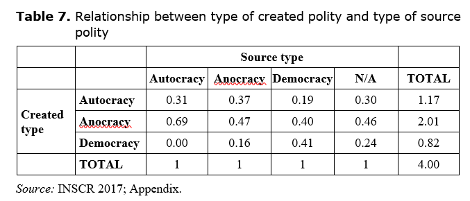
We see from Table 7 that a far higher proportion of polities created from democracies were themselves democracies than among polities created in other ways. A χ² analysis of the table rejects at the p < 0.01 level (p = 0.006) the hypothesis that the figures in each column are drawn from the same distribution. In other words, the difference between democracies and other types of source polity is significant. This suggests that a tendency to democracy did spread by inter-polity influence as would be expected for a global-level learning process.

We also see from Table 7 that polities not clearly originating from an identifiable source had a distribution almost identical to the overall distribution of newly created polities (compare the figures in column N/A of Table 7 with those in the rightmost column of Table 6). Hence polities with no definite antecedent experienced only generalised influence, while those that did have a definite antecedent were biased towards particular polity types by the nature of that antecedent. If we omit the N/A column and redo the χ² test focusing just on autocracies, anocracies and democracies, we find that the significance is strengthened to p = 0.001, indicating that, for those polities that had an antecedent, the different polity types indeed exerted significantly different influences on their daughter polities.

Of course, polities did not necessarily retain the type with which they came into existence. The spread of democracy has occurred not just through the creation of democracies but because polities of other types have changed into democracies. Furthermore, polities that were created as democracies may have reverted to anocracies or autocracies.

To understand the dynamics of political transformation, we need to investigate the properties of these transitions. For this purpose, each polity in the dataset was examined in every year. Its existing polity type was noted and then it was determined whether in the next year it remained the same or transitioned to another polity type. The numbers of each possible type of transition (including staying the same) were added up and in this way the annual probabilities for each polity type of staying the same or transitioning to another polity type were determined. The results are shown in Fig. 17 (omitting probabilities of staying the same, which can be deduced since probabilities must sum to 1).

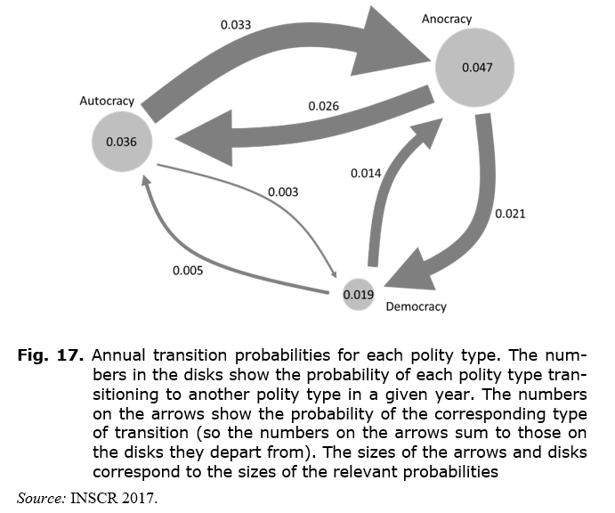
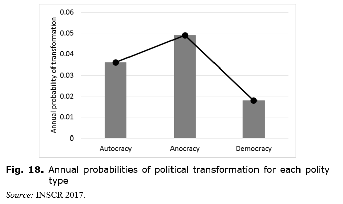
We find from Fig. 17 that anocracies were the most likely to undergo political transformation, with an annual probability of 0.049 of transitioning to either autocracy or democracy. This is also illustrated in Fig. 18. It recalls the familiar ‘inverted-U’ of political instability, whereby instability is lowest among the most and least autocratic regimes, and highest among the middling regimes, also with an asymmetry such that autocracies are less stable than democracies (Slinko et al. 2017). This is to be expected, since political transformation inherently implies instability of the preceding regime. Thus, we see that anocracies are most likely to transform, via either democratic revolution or autocratic takeover. Fig. 17 shows us that the two types of transformation are almost equally likely (probabilities of 0.026 to autocracy and 0.021 to democracy).

The fact that democracies are the most stable kind of polity reflects the ‘lock-in’ referred to above (see the discussion surrounding Fig. 9). Once polities have become democracies they tend to remain as such. Unlike anocracies and autocracies, whose numbers fluctuate, the number of democracies tends only to rise, in accordance with Modelski and Perry's (2002) learning process.

In the case of autocracies, we find that they are very unlikely to transition directly to democracies. They are ten times more likely (0.033 versus 0.003) to turn into anocracies. Once turned into anocracies, they then have roughly equal probabilities of reverting to autocracies or completing the transformation to democracies.[2]

If, as discussed above, fear is a factor in political transformation, we might expect such fear to be highest in anocracies. These polities are characterised by the highest incidences of strikes, riots, crises, demonstrations and guerrilla warfare, all of which are likely to induce a high sense of uncertainty and insecurity among the relevant populations (Slinko et al. 2017). These middling polities also tend to have middling prosperity, rather than people being reduced to the bare survival level, which is more common among autocracies (Korotayev et al. 2018; Korotayev, Bilyuga, and Shishkina 2018). Paradoxically, this middling prosperity may actually enhance the sense of economic insecurity, insofar as people have more to lose. ‘Cease to hope…and you will cease to fear’ (Seneca 1969: 38 [Letter 5]). Those who are still struggling to hold on to a decent way of life may experience more anxiety than those who have already lost everything. Thus, anocracies are characterised by unrest, conflict and the threat of financial ruin, so that people living in such polities experience elevated economic and political insecurity. Given that fear and insecurity make people more disposed to support authoritarian figures (see above), it is not surprising to find from Fig. 17 that anocracies are five times more likely to transition to autocracy than democracies are (0.026 versus 0.005).

Mathematical Analysis

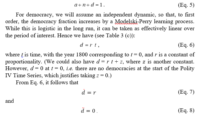
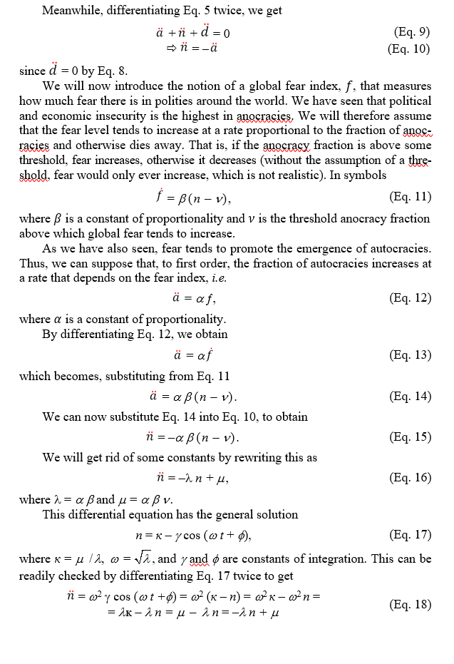
We are now in a position to develop a mathematical model to account for the first order dynamics of global political evolution. We will use the same symbols as above so that ,  and  represent the fractions of polities that are autocracies, anocracies and democracies respectively. We know that

Conclusion

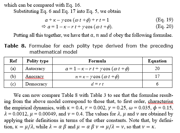
From the preceding analysis, the threshold anocracy fraction ( ) above which global fear begins to increase turns out to be 0.4 or 40 %. After this, as fear rises, we should eventually expect a turn towards extremism and authoritarianism, and therefore the proliferation of autocratic regimes. This threshold level was reached and exceeded during the second half of the 19^th century. From this perspective, and from the formulae of Table 8 / Table 3, the various brands of totalitarianism that emerged in the first half of the 20^th century had their primary origins not in the events of that time but in the political conditions of the late 1800s. This is ‘to first order’. It is not to deny that some of their specific features and nuances – the second-order characteristics – may have been shaped by more contemporary concerns.

Implicitly, since the populations of the late 19^th and early 20^th century belonged to different generations, there was some cultural lag in the propagation of fear and its effects. In fact, ‘human fears are most efficiently understood as social phenomena’ (Scruton 1986: 9, 15), as is exemplified by ‘moral panics’ and generally the transmission of fearfulness through social cues (Pain and Smith 2008: 9; Furedi 2007a). The growth of generalised societal fear is therefore not an instantaneous psychological reaction but a process of communication, transmission and reinforcement that builds up over time. In particular, parental generations may communicate fear to offspring generations, which then amplify and ultimately act upon it.

These observations alert us to the long-range nature of global political transformation. Conditions applying today may shape outcomes many decades in the future. With  = 0.035, the period of the autocracy-anocracy fluctuation turns out to be 180 years (= ), hence 90 years from peak to trough. Insofar as regime type is only one influence on a population's fear and insecurity, albeit an important one, a next step would be to extend the above mathematical model, particularly Eq. (11), to obtain a richer representation of fear dynamics and thus gain increased predictive power concerning the transformation of global politics in relation to instability, conflict and economic change.

In identifying the oscillatory pattern that has prevailed in the past and that, over the coming century, will begin to collide with the spread of democracy, as illustrated in Fig. 9, this model also alerts us to the fact that we ought to see growing distortions in this oscillation and its eventual breakdown. Whether we see such distortions and what form they take will help us determine whether democratic political institutions will continue to spread in the hopeful, end-of-history-like learning process described by Modelski and Perry, or whether resurgent instability and fear-inducing economic and other phenomena will lead future generations back to more authoritarian attitudes and political forms.

References

Bolt J., Timmer M., and van Zanden J. L. 2014. GDP per Capita since 1820. How Was Life? Global Well-being since 1820 / Ed. by J. L. van Zanden et al., pp. 57–72. Paris: OECD Publishing.

Center for Systemic Peace. n.d. The Polity Project. URL: http://www.systemicpeace.org/polityproject.html. Date accessed: 05.12.2019.

Corradi J. 1992. Toward Societies Without Fear. Fear at the Edge: State Terror and Resistance in Latin America / Ed. by J. Corradi et al., pp. 267–292. Oxford: University of California Press.

Furedi F. 2007. Towards a Sociology of Fear. Fear: Essays on the Meaning and Experience of Fear / Ed. by K. Hebblethwaite, and E. McCarthy, pp. 18–30. Dublin: Four Courts Press.

Integrated Network for Societal Conflict Research (INSCR). 2017. Polity IV Annual Time-Series, 1800–2017. URL: http://www.systemicpeace.org/inscrdata.html. Date accessed: 05.12.2019.

Korotayev A., Vaskin I., Bilyuga S., and Ilyin I. 2018. Economic Development and Sociopolitical Destabilization: A Re-Analysis. Cliodynamics 9: 59–118.

Korotayev A., Bilyuga S., and Shishkina A. 2018. GDP Per Capita and Protest Activity: A Quantitative Reanalysis. Cross-Cultural Research 52(4): 406–440.

McCartney C. 1991. Coming to Terms with Violence: Social Discourse in the Development of a Shared Ideology. The Irish Terrorism Experience / Ed. by Y. Alexander and A. O'Day, pp. 97–122. Aldershot: Dartmouth.

Merolla J., and Zechmeister E. 2009. Democracy at Risk: How Terrorist Threats Affect the Public. Chicago: University Press.

Modelski G., and Perry III G. 1991. Democratization in Long Perspective. Technological Forecasting & Social Change 39: 23–34.

Modelski G., and Perry III G. 2002. Democratization in Long Perspective Revisited. Technological Forecasting & Social Change 69: 359–376.

Muldoon O. 2003. The Psychological Impact of Protracted Campaigns of Political Violence on Societies. Terrorists, Victims, and Society: Psychological Perspectives on Terrorism and its Consequences / Ed. by A. Silke, pp. 161–174. Chichester: Wiley.

Pain R., and Smith S. 2008. Fear: Critical Geopolitics and Everyday Life. Aldershot: Ashgate.

Pozrvanović M. 1993. Culture and Fear: Everyday Life in Wartime. Fear, Death, and Resistance: An Ethnography of War: Croatia, 1991–1992 / Ed. by L. Čale Feldman, I. Prica, and R. Senjković, pp. 119–150. Zagreb: Institute of Ethnology and Folklore Research.

Scruton D. 1986. The Anthropology of an Emotion. Sociophobics: The Anthropology of Fear / Ed. by D. Scruton, pp. 1–6. London: Westview.

Seneca L. 1969. Letters from a Stoic. Transl. by R. Campbell. Harmondsworth: Penguin.

Slinko E., Bilyuga S., Zinkina J., and Korotayev A. 2017. Regime Type and Political Destabilization in Cross-National Perspective: A Re-Analysis. Cross-Cultural Research 51(1): 26–50.

Smallman S. 2002. Fear and Memory in the Brazilian Army and Society, 1889–1954. London: University of North Carolina Press.

Appendix

This Appendix identifies the states from which polities created after 1800 broke away. Although there are no doubt errors and arguable elements in this listing, it is believed robust enough to support the key conclusion, namely that breakaway polities were more likely to be democracies when they arose from democracies.

Polity	Creation date	Origin
Albania	1914	Turkey
Algeria	1962	France
Angola	1975	Portugal
Argentina	1825	Spain
Armenia	1991	The USSR
Australia	1901	The United Kingdom
Azerbaijan	1991	The USSR
Baden	1819	N/A
Bahrain	1971	The United Kingdom
Bangladesh	1972	Pakistan
Belarus	1991	The USSR
Belgium	1830	The Netherlands
Benin	1960	France
Bhutan	1907	N/A
Bolivia	1825	Spain
Bosnia	1992	Austria-Hungary
Botswana	1966	The United Kingdom
Brazil	1824	Portugal
Bulgaria	1879	Turkey
Burkina Faso	1960	France
Burundi	1962	Belgium
Cambodia	1953	France
Cameroon	1960	France
Canada	1867	The United Kingdom
Cape Verde	1975	Portugal
Central African Republic	1960	France

Continuation of Table

Polity	Creation date	Origin
Chad	1960	France
Chile	1818	Spain
Colombia	1832	Spain
Comoros	1975	France
Congo Brazzaville	1960	France
Congo Kinshasa	1960	Belgium
Costa Rica	1838	Spain
Cote D'Ivoire	2016	France
Croatia	1991	Yugoslavia
Cuba	1902	Spain
Cyprus	1960	United Kingdom
Czech Republic	1993	Czechoslovakia
Czechoslovakia	1918	Austria-Hungary
Djibouti	1977	France
Dominican Republic	1844	Haiti
East Timor	2002	Indonesia
Ecuador	1830	Spain
Egypt	1922	The United Kingdom
El Salvador	1841	Spain
Equatorial Guinea	1968	Spain
Eritrea	1993	Ethiopia
Estonia	1917	Russia
Ethiopia	1993	N/A
Fiji	1970	The United Kingdom
Finland	1917	Russia
Gabon	1960	France
Gambia	1965	The United Kingdom
Georgia	1991	The USSR
Germany	1868	N/A
Germany East	1945	N/A
Germany West	1945	N/A

Continuation of Table

Polity	Creation date	Origin
Ghana	1960	The United Kingdom
Gran Colombia	1821	Spain
Greece	1827	Turkey
Guatemala	1839	Spain
Guinea	1958	France
Guinea-Bissau	1974	Portugal
Guyana	1966	The United Kingdom
Haiti	1820	France
Honduras	1839	Spain
Hungary	1867	N/A
India	1950	The United Kingdom
Indonesia	1945	Netherlands
Iraq	1924	The United Kingdom
Ireland	1921	United Kingdom
Israel	1948	N/A
Italy	1861	N/A
Ivory Coast	1960	France
Jamaica	1959	The United Kingdom
Jordan	1946	The United Kingdom
Kazakhstan	1991	The USSR
Kenya	1963	The United Kingdom
Korea North	1948	The USSR
Korea South	1948	N/A
Kosovo	2008	Serbia
Kuwait	1963	The United Kingdom
Kyrgyzstan	1991	The USSR
Laos	1954	France
Latvia	1920	The USSR
Lebanon	1943	France
Lesotho	1966	The United Kingdom

Continuation of Table

Polity	Creation date	Origin
Liberia	1847	N/A
Libya	1951	Italy
Lithuania	1918	N/A
Luxembourg	1867	N/A
Macedonia	1991	Yugoslavia
Madagascar	1960	France
Malawi	1964	The United Kingdom
Malaysia	1957	The United Kingdom
Mali	1960	France
Mauritania	1960	France
Mauritius	1968	The United Kingdom
Mexico	1822	Spain
Modena	1815	Napoleonic Empire
Moldova	1991	The USSR
Mongolia	1924	China
Montenegro	2006	Serbia
Mozambique	1975	Portugal
Myanmar (Burma)	1948	The United Kingdom
Namibia	1990	South Africa
The Netherlands	1815	France
New Zealand	1857	The United Kingdom
Nicaragua	1838	Spain
Niger	1960	France
Nigeria	1960	The United Kingdom
Norway	1814	Sweden
Orange Free State	1854	The United Kingdom
Pakistan	1947	The United Kingdom
Panama	1903	Spain
Papal States	1815	Napoleonic Empire
Papua New Guinea	1975	Australia

Continuation of Table

Polity	Creation date	Origin
Paraguay	1811	Spain
Parma	1815	Napoleonic Empire
Peru	1821	Spain
Philippines	1935	The United States
Poland	1918	N/A
Qatar	1971	The United Kingdom
Romania	1859	N/A
Rwanda	1961	Belgium
Sardinia	1815	N/A
Saudi Arabia	1926	Turkey
Saxony	1806	Holy Roman Empire
Senegal	1960	France
Serbia	1830	Turkey
Serbia and Montenegro	2003	N/A
Sierra Leone	1961	The United Kingdom
Singapore	1959	The United Kingdom
Slovak Republic	1993	Czechoslovakia
Slovenia	1991	Yugoslavia
Solomon Islands	1978	The United Kingdom
Somalia	1960	Italy
South Africa	1910	The United Kingdom
South Sudan	2011	Sudan
Sri Lanka	1948	The United Kingdom
Sudan	1956	The United Kingdom
Sudan-North	2011	N/A
Suriname	1975	Netherlands
Swaziland	1968	The United Kingdom
Switzerland	1848	N/A
Syria	1944	France
Taiwan	1949	China

Continuation of Table

Polity	Creation date	Origin
Tajikistan	1991	The USSR
Tanzania	1961	The United Kingdom
Timor Leste	2016	N/A
Togo	1960	France
Trinidad and Tobago	1962	The United Kingdom
Tunisia	1959	France
Turkmenistan	1991	The USSR
Tuscany	1815	Napoleonic Empire
Two Sicilies	1816	Napoleonic Empire
UAE	1971	The United Kingdom
Uganda	1962	The United Kingdom
Ukraine	1991	The USSR
United Province CA	1824	N/A
Uruguay	1830	Brazil
The USSR	1922	N/A
Uzbekistan	1991	The USSR
Venezuela	1830	Gran Colombia
Vietnam	1976	France
Vietnam North	1954	N/A
Vietnam South	1955	N/A
Yemen	1990	N/A
Yemen North	1918	Turkey
Yemen South	1967	The United Kingdom
Yugoslavia	1921	Austria-Hungary
Zambia	1964	The United Kingdom
Zimbabwe	1970	The United Kingdom

---

[1] Specifically, the adjusted R-squared is given by where R² is the normal R-squared value, n is the number of data points and p is the number of free parameters.

[2] This point neglects memory effects, which have not been investigated. Thus a polity's history might affect its transition probabilities, such that say polities that have been autocracies before are more likely to become autocracies again. However, since many more anocracies come from autocracies than from democracies, whereas the probabilities of transition from anocracies to autocracies or democracies are roughly equal, any such bias cannot be particularly strong.