Hyperbolic Growth of the Human Population of the Earth: Analysis of Existing Models

Almanac: Globalistics and Globalization Studies
This work focuses on: 1) demographic problems arising from the growing human population of the Earth, and 2) on the quantitative estimates of the future growth of the Earth's population. We discuss the existing models of the global human population growth using a popular presentation level and without appealing to sophisticated mathematical language. Instead of proposing a new mathematical model of the population growth, we advance a new perspective for the mathematical modeling: phase transitions which are well-know in physics. In particular, we demonstrate that the world's demographic transition is actually a phase transition that has been affecting all aspects of our life.
Keywords: demographic transition, phase transition, world population.
Introduction
A. Empirical Models
The human population of the Earth, NE, attracted much attention after publication of the seminal work of Malthus who realized that it should exhibit the unlimited exponential growth:
 .
. The fears were partially dispersed by Verhulst who introduced the logistic equation,
to account for the population dynamics of closed communities. Here, r is the growth rate and K is the carrying capacity. This equation accounts fairly well for the growth of small communities but it fails to describe the long-time dynamics of the human population of the Earth.
As it was shown in the seminal work of von Foerster et al. (von Foerster, Mora, and Amiot 1960), the available to them data could be fairly well described by the empirical dependence

where a ≈ 1, C = 1.8 1011, and tc = 2026. The corresponding growth rate is:
The most striking feature of Eqs 3, 4 is the divergence of NE and dNE/dt at finite time tc. This indicates that the above equations are inappropriate in the vicinity of tc. Indeed, since 1960, the global human population growth has been deviating from the hyperbolic dependence indicated by the Eqs 3, 4; in particular, the growth rate NE–1dNE/dt achieved its maximum value of ~ 2.1 % in 1962 and then decreased steadily. This prompted the search for the functions that approximate the hyperbolic dependence given by Eqs 3, 4 before 1960 and replace them by smoother dependences after 1960. Several empirically found replacements have been suggested, including hypergeometric (Koronovskii 2000), overlay of several exponential or logistic curves (Hanson 1998), hyperexponential (Varfolomeev and Gurevich 2001), delayed logistic curves (Haberl and Aubauer 1992; Yukalov, Yukalova, and Sornette 2009), and others. The most insightful empirical approach was suggested by Kapitza (1996) who modified the Eq. 3 as follows:
Here, τ is a microscopic time scale for which Kapitza took the lifespan of a generation, ~ 45 years. This modification captures the maximum in the relative growth rate and assumes that the human population eventually comes to saturation. The subsequent studies sought to justify this empirical approach.
B. Mathematical Models
Models considering the carrying capacity of the Earth
In order to understand the future trends of the global human population growth, several non-empirical mathematical models have been developed. These models aimed to derive Eqs 3, 4 from the ‘first principles’. This approach implies that Eqs 3, 4 are consequences of some plausible scenario while the parameters of these equations are still empirical. Most of such models (Artzrouni and Komlos 1985; Cohen 1995; Kremer 1993; Komlos and Nefedov 2002; Podlazov 2004; Galor and Moav 2001; Korotayev, Malkov, and Khaltourina 2006) quantified the verbal approach of Boserup, Simon, Jones, etc. who attributed the accelerating growth of the human population of the Earth, NE, to positive feedback between the population size and the Earth's carrying capacity, KE. Then, in addition to Eq. 2 which accounts for the fast growth of the world population, these models introduced an additional equation that accounts for the slow dynamics of the population growth resulting from the gradual increase of the carrying capacity:

The coefficient γ quantifies the rate with which the human race expands the carrying capacity of the Earth. In such a way, these models assume two rates of the population growth. The fast rate, as derived from Eq. 2, is N–1dN/dt ~ r; while the slow rate, as derived from the Eq. 6, is K–1dK/dt ~ γN. As far as r >> γN the instantaneous value of the population size is N ≈ K (see Eq. 2, the index E has been omitted). Then Eq. 6 reduces to

This equation describes an autocatalytic process and its solution is given by Eq. 3, where C = 1/γ, tc = ti + 1/γNi and ti, Ni are initial conditions. Upon approaching tc, the population size N increases and the distinction between the slow and fast dynamics eventually disappears. In the limit γN >> r, the Eqs 2, 6 yield exponential population growth, N ~ ert.
At present we do not know whether the human population will come to saturation in future or will grow continuously, although we want to believe that its growth will be somehow limited. The Kapitza's conjecture consists in replacing the Eq. 7 by the empirical equation
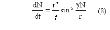
that describes accelerating and then decelerating population growth, whereas the population size is eventually stabilized at Ninfty = pr/γ. Eq. 8 describes the dynamic crossover. It operates with the minimal number of parameters: r and γ, and it is mathematically appealing. However, this equation cannot be easily justified and the reasons for the maximum of the growth rate and for the stabilization of the population size remain obscure.
Models based on the Gross Domestic Product-GDP
The carrying capacity, being an important parameter of the demographic models, can not be measured directly. The model that does not consider explicitly the carrying capacity was developed by Kremer (1993) who considered the gross domestic product, GDP = N(S + m), as the key parameter that determines the slow dynamics of the population growth. Here, N is the population size, m is the subsistence level, and S is the surplus product. Kremer related the GDP to the level of technological development T as follows: GDP ~ Nf1Tf2, where f1,f2 are the exponents that should be found empirically. In fact, Kremer put onto quantitative language the verbal approach that had been developed earlier by Kuznets, Boserup, Jones, etc. The key assumption of the Kremer's model is that the growth of GDP is spurred by the technology growth.
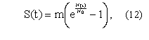
The original model developed by Kremer is static while Korotayev, Malkov and Khaltourina (2006) developed a family of dynamic models basing on Kremer's ideas. In the framework of these models, the dynamic variable that quantifies the technological development is the surplus product, S. The simplest model considered by Korotayev, Malkov and Khaltourina consists of two equations:
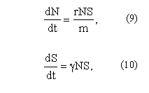
with two empirical parameters: r is the rate of the population growth, and γ has now the meaning of the average creative ability of a person. The parameter m characterizes the scale of the surplus product S (it can be chosen to be equal to subsistence level) and it has been introduced here to be consistent with the notation of the Eq. 1. In such a way, the Eq. 9 is the modification of the Eq. 1, while Eq. 10 captures the Kremer's idea. The relation to Kremer's work is even more evident if we notice that for f1 ~ 1 the definition of the technological level by Kremer: T ~ (GDP/N)1/f2 is closely related to the definition of the surplus product: (S + m) ~ GDP/N.
The relation between N and S can be found by dividing Eq. 9 by Eq. 10. This yields N ~ S. In other words, Eqs 9, 10 describe the positive feedback between the surplus product and the population growth, on the one hand; and the positive feedback between the increasing population and the growth of the surplus product, on the other hand.[1] The solution of these equations exhibits finite-time singularity for N(t) and S(t).
The field of applicability of Eqs 9, 10 is evident from their very structure: the right side looks as if it were the first term of the power series in the small parameter S/m. In other words, Eqs 9, 10 assume that S/m << 1, that is they should describe the period before 1870 when S/m = 1. One can go beyond this approximation and modify the Eqs 9, 10 to extend their applicability range above the year 1870. Indeed, if we assume that the surplus product goes to creation of new working places, the relation of carrying capacity to surplus product is especially simple: K = GDP/m = N(S/m + 1). We replace Eq. 9 by the logistic equation Eq. 2, where K has been expressed through S and find
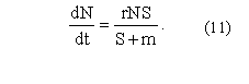
This equation introduces negative feedback between the population growth and the growing population. This has some stabilizing effect and consequently, the solution of Eqs 10, 11 does not diverge. In the long run, the growth rate of N comes to saturation, while the growth rate of S is unlimited. The relation between N and S can be found by dividing Eq. 10 by Eq. 11. This yields 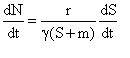 . The solution of this equation is
where N0 = const. In what follows we analyze the relative growth rates: rN = dN/dt : N and rS = dS/dt : S and compare them to the prediction of Eqs 10–12.
Fig. 1 shows that the relation between N and S is superlinear and is fairly well described by Eq. 12 with N0 = 1.65 · 109, the agreement breaks only for N > 3 · 109 (this corresponds to years 1960–1970).
Fig. 2 shows that the human population growth rate linearly increases with N, achieves its maximum value of rNmax = 0.021 at N ≈ 3 109 and then starts to decrease. Equation 11 correctly predicts dynamics of rN at N < 2 · 109 and deviates from the actual data at higher N.
Fig. 1. Relation between the surplus product S/m and the World human population N in the same year
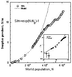
Notes: The circles show the data taken from the US Census database, Maddison (2001), Kremer (1993). The subsistence level is m = 440$ USD. The dashed line is the prediction of Eq. 12 with N0 = 1.65 · 109. The inset shows the same data in the log-log scale.
Fig. 2. World population growth rate, rN = dN/dt : N
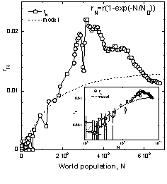
Notes: The circles show the data taken from the US Census database, Maddison (2001), Kremer (1993). The dashed line is the prediction of Eq. 11 with N0 = 1.65 109 and r = 0.013. The inset shows the same data in the log-log scale.
Fig. 3 shows that the World surplus product growth rate linearly increases with N, achieves its maximum value of rSmax = 0.04 at N ≈ 3 · 109 and then starts to decrease. Equation 10 correctly predicts dynamics of rS at N < 2 · 109 and deviates from the actual data at higher N. We conclude that the Eqs 10, 11 extend the range of applicability of the Korotayev, Malkov, and Khaltourina model from the year ~1870 to the year ~1960. Since no new parameters/variables have been introduced, this extension belongs to the same family of models.
Fig. 3. World surplus product growth rate, rS=dS/dt : S
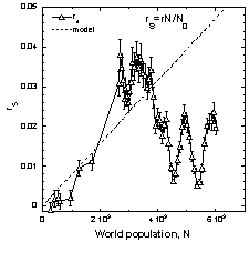
Notes: The circles show the data taken from Maddison (2001). The subsistence level is m = 440$ USD. The data were averaged over the five-year interval. The dashed line shows prediction of Eq. 10 with N0 = 1.65 · 109.
Fig. 4 shows the population growth rate rN and the surplus product growth rate rS versus surplus product, S/m. Both rN and rS grow with S, achieve the maximum at S/m ~ 5−6 (this corresponds to N ≈ 3 · 109) and then decrease. The model correctly predicts initial increase of rN and rS with S (that corresponds to S/m < 1) while pronounced deviations from the model occur for S/m > 2.
Fig. 4. Comparison of the world population and the world surplus product growth rates
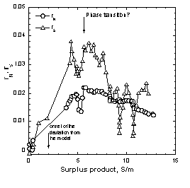
Notes: The data for rS were averaged over the five-year interval. Notice that maximum rN and maximum rS are achieved simultaneously, at the same value of S/m.
Models accounting for the demographic transition
The maximum in the population growth rate (Fig. 2) is usually associated with the ‘demographic transition’ (Chesnais 1992) which results from the decrease of mortality rate and the subsequent birth rate decrease. Detailed statistical studies indicate that the reason for decreasing population growth in developed countries nowadays is the declining birth rate (Ibid.) whereas there is a strong anticorrelation between the level of female education and fertility. Korotayev, Khaltourina and Malkov captured this by introducing an additional dynamic variable: the fraction of literate population, l. They modified the Malthus equation (Eq. 9) to account for the negative feedback between the population growth and the literacy level:

The dynamics of the surplus product remained the same (Eq. 10) while the dynamics of l has been described by the following equation:

where a is a new empirical parameter and S is dimensionless (it can be measured in the units of subsistence level, m). When the initial educational level of the population is low, this model predicts accelerating growth of N, S, and l. Eventually, when l comes to saturation, N also achieves saturation while S does not saturate and grows exponentially. Therefore, this extended model captures the non-monotonous dependence of rN on N (Fig. 2) but fails to account for the non-monotonous dependence of rS on N (Fig. 3).
Critical assessment of the above models
The common feature of all previously discussed models is that they describe the growth of the world human population growth, GDP, surplus product, literacy, etc. by using ordinary differential equations containing first-order time derivatives. In the framework of these models, the non-monotonous time dependence of the growth rate (demographic transition) results from the dynamic crossover, that is at all times there are several factors affecting population growth and these factors operate simultaneously. With a small population number, N < 3 · 109, one factor wins and the growth rate increases with N; while for a high population number, N > 3 · 109, another factor wins and the growth rate decreases with N. When N ≈ 3 109, the gradual transition from one regime to another occurs.
Several features in real data challenge this picture. First, the transition from increasing to a decreasing trend in rN versus N dependence is very sharp (Fig. 2). Second, it is not clear why transitions in rN and rS occur simultaneously in 1960–1970, and at the same value of N ≈ 3 ·109 (Fig. 4). Other parameters also undergo especially fast change in the same time period – 1960–1970; these include age structure of the population, the level of literacy, urbanization (Korotayev, Malkov, and Khaltourina 2006), financial indices (Johansen and Sornette 2001), etc. All these features are more naturally accounted for from another perspective – phase transition. While the commonly accepted approaches (Korotayev, Malkov, and Khaltourina 2006) focus on time-dependent, dynamic properties of the population growth, the phase transition approach focuses on how demographic and economic variables depend on control parameters such as population or surplus product.
Is Demographic Transition a Phase Transition?
The notion of phase transition has been developed in the context of condensed matter physics. In the system of many interacting particles/agents, when the control parameter (temperature, pressure, density, etc.) varies, the system can progress abruptly from the disordered phase where the radius of correlations is finite, to the ordered phase, which is characterized by the long-range order. This situation can be usually described using the order parameter which is zero in the disordered phase and non-zero in the ordered phase. The properties of the system as a function of the control parameter are frequently non-analytic at the transition point. In particular, the correlation length diverges upon approaching the phase transition and becomes infinite in the ordered phase. Divergence of many physical properties at the phase transition is related to the divergence of the correlation length. The dynamic properties also undergo dramatic changes and the fluctuations grow on the both sides of the phase transition (Stanley 1999). The difference between the phase transition and crossover scenario is in the following: for the former, the ordered state is characterized by an emerging new property – the order parameter (which was absent in the disordered state); while for the latter scenario all factors were present in both states.
Phase transitions in social systems such as financial markets, traffic flow, etc., were noticed long ago (Montroll 1978; Montroll and Badger 1975; Stauffer and Solomon 2009). The extrapolated divergence of the human population growth rate in 2026–2040 has been also interpreted as some kind of transition (von Foerster, Mora, and Amiot 1960; Korotayev, Malkov, and Khaltourina 2006; Johansen and Sornette 2001). However, the growth rate divergence appears only in the ‘mean-field’ models. More realistic models lift the divergence and yield earlier date for the population growth to switch from one regime to another. This probably implies that the phase transition has already taken place in 1960–1970, rather than to occur in 2026–2040. Then the demographic transition of 1960–1970 is not a purely demographic phenomenon but is a signature of the global phase transition that has been affecting all aspects of human life.
It is instructive to discuss the properties of this transition in the context of such a generic phase transition as lattice percolation (Stauffer and Aharoni 1994). Here, the disordered state contains disconnected finite-size clusters while the ordered state is characterized by the appearance of the infinite cluster that ensures connectivity of the whole system. This analogy prompts us to consider globalization as a hallmark of the phase transition of 1960–1970. One of the most prominent aspects of globalization is the economic integration. We consider a very crude indicator of the economic integration – the growth of the European Union, in particular we focus on η = NEU / NEurope – the fraction of the European population in the states belonging to European Union or to its predecessors such as the Common Market.
Fig. 5 shows dynamics of η. Amusingly, this very simple measure of the European integration mimics the World Globalization index as determined by Dreher (2006) using weighted economic, political and cultural indicators. Fig. 5 shows that the onset of European integration took place in the same period – in 1960–1970 – when the global demographic transition occurred. Serrano (2007) came earlier to similar conclusions by considering the historical dynamics of bilateral trade balance. Dependence η (t) is very similar to the behavior of order parameter at the percolation phase transition (Stauffer and Aharoni 1994).
Fig. 5. Dynamics of the European Union growth, η = NEU / NEUROPE and of the KOF globalization index
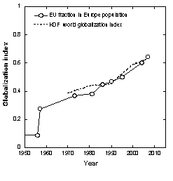
Notes: The circles show NEU , the population in the states that belong to the European Union or to its predecessors (Common Market), while NEUROPE is the total European population. The dashed line shows KOF globalization index (Dreher 2006). Note abrupt growth of η around 1960 which is followed by slower steady growth afterwards. This reminds a characteristic behavior of the order parameter at phase transitions.
If we adopt the hypothesis of the humanity as a system of interacting agents that undergoes instability/phase transition with a peak in 1960–1970, this raises many interesting questions that prompt extensive scientific research.
· What is the nature of the phase transition? What is the difference between two phases? Probably, in the years preceding 1960–1970, the most part of the surplus product eventually went to the population growth. However, after 1960–1970 the surplus product was spent more on the increase of the quality of living, i.e. it was channeled to the increase of subsistence level.
· What is the proper control parameter that drives this phase transition? Is it the total human population, or average population density, or surplus product, or something else?
· What is the order parameter? Globalization index? Another candidate for the order parameter could be some measure of information since the appearance of the global information network (Kapitza 1996; Dolgonosov and Naidenov 2006) after 1970 was very prominent.
· Which parameters diverge upon approaching the transition? What are the critical indices? Besides urbanization and literacy that were studied by Korotayev, Malkov and Khaltourina (2006) it would be interesting to consider the historical dynamics of the warfare indicators such as the weapon range, the power of the explosives, etc.
· How one can define the correlation length? The possible candidates could be the average city population (Chase-Dunn and Manning 2002) or the average size of a polity (Taagepera 1997).
· What is the statistics of fluctuations at this transition? It is well-known that the fluctuations grow upon approaching the phase transition from both sides. The growth of fluctuations in the context of global population growth has been already noticed (Johansen and Sornette 2001). In this context, it would be especially interesting to consider the timeline of the financial crises.
· What is the behavior of the dynamic properties of the global human population at the transition? The analog of conductivity of the percolating network would be the signal propagation rate or the rate of adoption of technological innovations. How did these parameters change through historical time?
Spatially-inhomogeneous and discrete models
Our capability to introduce innovations that enlarge carrying capacity of the Earth (autocatalycity) translates into human population dynamics equations as a positive feedback. It is well known that population dynamics that includes positive feedback and diffusion leads to strongly spatially-inhomogeneous population pattern (for example, desert oases, vegetation patches in arid zones [Shnerb, Sarah et al. 2003], etc.) and favors agglomeration. Indeed, the increasing economic returns and increasing innovation rate arising from the population agglomeration in cities is well documented (Bettencourt et al. 2007). This means that in the context of the human population dynamics, the spatial heterogeneity by itself has autocatalytic properties. Therefore, the models of the human population dynamics should properly address the spatial dimension.
Note also that the previously discussed models were based on ordinary differential equations, as it is commonly accepted in population dynamics (Turchin 2001), and took into account neither spatial distribution of the population nor the discrete nature of humans. Very often when the continuum equations describing population dynamics assume spatially homogeneous population and predict a very slow growth or even population extinction; the individuals self-organize in spatio-temporally localized adaptive patches which ensure their survival and development. In other words, continuum differential equations may fail in predicting the population dynamics of the discrete proliferating agents (Shnerb, Louzoun et al. 2000). An interesting example of such approach is the recent study of the economics development in Poland after 1990 (Yaari et al. 2008). Yaari et al. showed that the economics growth was led by few singular ‘growth centers’ that were associated with the University centers. Probably, this shows in a different way the ultimate relation between the education level/literacy and the human population dynamics (see Korotayev, Malkov, and Khaltourina 2006). All this calls for new generation of the models describing the world human population growth. These should be discrete and spatially-inhomogeneous models.
Physical Meaning of the Parameters of the Dynamic Models
We consider here a different subject that emerges in relation to dynamical models of the human population growth. Eqs 10, 11 contain two empirical parameters: r, γ that should be somehow related to the human nature. The meaning of the parameter r is more or less clear – it is the relaxation rate of the population to sudden changes. It is determined by the difference in birth rate and mortality and, to the best of our knowledge, does not exceed rrecord = 0.14. Comparison of the growth rate to the models (Fig. 2) yields r = 0.01 ~ 0.1 rrecord that is quite reasonable. Note, that r can be measured from the transient phenomena, for example, how fast the population size recovers from dramatic disaster such as WWII. This yields r ~ 0.02–0.03 that is comparable to r = 0.013 determined from the Fig. 2.
The meaning of the parameter γ is more elusive. Kapitza (1996) suggested that γ = 1/rU2 where U ≈ 67,000 is the coherent population unit. This implies a paradoxical conclusion that any coherent population unit consisting of ~ 67,000 individuals will develop into civilization consisting of billions of individuals. To get more clear insight into this paradox we compare the humans to the beavers. Besides their short lifespan (16–20 years), the beavers remind humans in several aspects: they are monogamous, they live in colonies, and most important – by building the dams they shape the landscape according to their needs, i.e. they can expand the carrying capacity. However, the difference between the ‘civilization’ of beavers and human civilization is too obvious. Hence, we seek for the deeper relation between the parameter γ and the human nature.
Korotayev, Malkov and Khaltourina (2006) related γ to the average creativity of a person. To elaborate further on this subject we assume the following scenario. Human population N adjusts to the current carrying capacity very fast. Carrying capacity K slowly increases due to technological innovations. So far, the spreading of the technological innovations has been the bottleneck that determined the dynamics of the carrying capacity growth. Eq. 6 can be recast as follows:

where Nt is the total number of humans lived on the Earth till time t, and τ is the average lifetime of the generation. The solution of Eq. 15 is K = Kiexp(γτNt) where Ki is the carrying capacity at time ti and Nt is the total number of humans that lived on Earth between ti and t. Then

For the hyperbolic population growth (Eqs 3, 4), the total number of people lived between ti and t depends logarithmically on time:

The technological innovations are created by people and they are accumulating. This means that the carrying capacity at time t is the result of activity of all people that lived before (Cohen 1995). Therefore, the parameter γτ characterizes the average contribution of an individual to the expansion of the carrying capacity of the Earth. This may be interpreted in two ways.
1. Each individual contributes to the growth of the Earth carrying capacity in such a way that the average personal contribution, ΔK = γτK.
2. The carrying capacity increases by abrupt steps, ΔK ~ K, due to stepwise development of science (Turchin 1977) and to scientific/technological revolutions (Kuhn 1962). Then γτ is the probability/frequency of these technological revolutions. These revolutions are rare events that trigger a series of smaller innovations which become embodied long before the next revolution occurs. According to this interpretation, the parameter γτ is the probability that an inventor or group of inventors makes a major technological/social/administrative breakthrough. According to this scenario, the human population growth is a series of logistic curves, each corresponding to a technological revolution. The quantity N0 ≈ 1/γτ (see Eq. 12) has the meaning of the number of people lived that ensure one major technological revolution.
We believe that the second scenario is more adequate. It has several implications:
· Log-periodic oscillations around hyperbolic law given by Eq. 3 which were noticed by several groups (Korotayev, Malkov, and Khaltourina 2006; Johansen and Sornette 2001) and attributed to cycles, correspond to major technological revolutions.
· The current demographic transition and deviation from the hyperbolic law appear when the technological revolutions occur so frequently that the full potential of the preceding revolution has not been fully realized before the next one occurs.
· While the motivation for technological innovations so far was the drive towards increasing carrying capacity, now something changed and the stream of innovations results in increased quality of living rather than in increasing number of living persons. (This is probably equivalent to increasing subsistence level m.) Hence, the population growth is not so fast.
· Is it possible that the very small probability γτ ≈ 10–9 is somehow related to the frequency of genetic mutations which is also exceedingly small (10–7–10–8)?
· The observation that bigger populations develop fast, while isolated continents, archipelagos and islands develop slower may be explained quite naturally. This should be related to the probability of appearance of rare events and innovators, and to the discreteness of the population.
The link between the above description and that of Kapitza (1996) is provided by the discrete character of humans. Indeed, to initiate the positive feedback loop given by Eq. 6 for the initial group of hominids to expand, it should create at least one working place in the lifetime of one generation. This brings us to the minimal group size of Ni ~ (γτ)–1/2 ~ 67,000.
Another consequence of the approach based on the number of people lived in the certain time interval, is the meaning of ‘historical time’. It has been already noticed (Kapitza 1996) that with respect to the frequency of historical events, the natural time scale is logarithmic rather than linear. Since the total number of humans that lived on the Earth also depends logarithmically on time (Eq. 17), then Nt seems to be the ‘internal clock’ of humanity. This conjecture provides the basis for quantitative comparison of the historical development of different isolated communities. According to this interpretation, the internal clock of a community is the total number of people that ever lived in this community.
Acknowledgments
I am grateful to Sorin Solomon for encouragement and for stimulating discussions.
References
Artzrouni, M., and Komlos, J. 1985. Population Growth through History and the Escape from the Malthusian Trap: A Homeostatic Simulation Model. Genus 41 (3–4): 21–39.
Bettencourt, L. M. A., Lobo, J., Helbing, D., Kuhnert, C., and West, G. B. 2007. Growth, Innovation, Scaling and the Pace of Life in Cities. PNAS 104: 7301–7306.
Chase-Dunn, C., and Manning, S. 2002. City Systems and World Systems: Four Millennia of City Growth and Decline. URL: http:/repositories.odlib.org/irows/ccr021.
Chesnais, J. C. 1992. The Demographic Transition: Stages, Patterns and Economic Implications. Oxford: Clarendon Press.
Cohen, J. E. 1995. Population Growth and Earth's Carrying Capacity. Science 269(5222): 341–346.
Dolgonosov, B. M., and Naidenov, V. I. 2006. An Informational Framework for Human Population Dynamics. Ecological Modeling 198: 375–386.
Dreher, A. 2006. Does Globalization Affect Growth? Evidence from a New Index of Globalization. Applied Economics 38: 1091–1110. URL: http://globalization. kof.ethz.ch/.
Foerster, H. von, Mora, P., and Amiot, L. 1960. Doomsday: Friday, 13 November, A. D. 2026. Science 132: 1291–1295.
Galor, O., and Moav, O. 2001. Natural Selection and the Origin of Economic Growth, Evolution and Growth. European Economic Review 45: 718–729.
Haberl, H., and Aubauer, H. P. 1992. Simulation of Human Population Dynamics by a Hyperlogistic Time-Delay Equation. Journal of Theoretical Biology 156: 499–511.
Hanson, R. 1998. Long-Term Growth as a Sequence of Exponential Modes. URL: http://hanson. gmu.edu/longgrow.pdf.
Johansen, A., and Sornette, D. 2001. Finite-Time Singularity in the Dynamics of the World Population, Economic and Financial Indices. Physica A 294: 465–502.
Kapitza, S. P. 1996. The Phenomenological Theory of the World Population Growth. Uspehi Fizicheskih Nauk 166(1): 63–80.
Komlos, J., and Nefedov, S. 2002. A Compact Macromodel of Pre-Industrial Population Growth. Historical Methods 35: 92–94.
Koronovskii, A. A. 2000. Population Dynamics as a Process Obeying the Nonlinear Diffusion Equation. Doklady Earth Sciences 372 (4): 755–758.
Korotayev, A., Malkov, A., and Khaltourina, D. 2006. Introduction to Social Macrodynamics: Compact Macromodels of the World System Growth. Moscow: URSS.
Kremer, M. 1993. Population Growth and Technological Change: One Million B. C. to 1990. The Quarterly Journal of Economics 108: 681–716.
Kuhn, T. S. 1962. The Structure of Scientific Revolutions. Chicago, IL: University of Chicago Press.
Maddison, A. 2001. Monitoring the World Economy: A Millennial Perspective. Paris: OECD.
Montroll, E. W. 1978. Social Dynamics and the Quantifying of Social Forces. PNAS 75 (10): 4633–4637.
Montroll, E. W., and Badger, W. W. 1975. Introduction to Quantitative Aspects of Social Phenomena. New York: Gordon and Breach.
Podlazov, A. V. 2004. Theory of the Global Demographic Process. In Dmitriev, M. G., and Petrov, A. P. (eds.), Mathematical Modeling of Social and Economic Dynamics (pp. 269–272). Moscow: Russian State Social University.
Serrano, M. A. 2007. Phase Transition in the Globalization of Trade. Journal of Statistical Mechanics: Theory and Experiment L01002. DOI: 10.1088/1742-5468/2007/01/L01002
Shnerb, N. M., Louzoun, Y., Bettelheim, E., and Solomon, S. 2000. The Importance of Being Discrete: Life Always Wins on the Surface. PNAS 97 (19): 10322.
Shnerb, N. M., Sarah, P., Lavee, H., and Solomon, S. 2003. Reactive Glass and Vegetation Patterns. Physical Review Letters 90: 0381011.
Stanley, H. E. 1999. Scaling, Universality, and Renormalization: Three Pillars of Modern Critical Phenomena. Reviews of Modern Physics 71: S358.
Stauffer, D., and Aharoni, A. 1994. Introduction to Percolation Theory. London: Taylor and Francis.
Stauffer, D., and Solomon, S. 2009. Physics and Mathematics Applications in Social Science. In Meyers, R. A. (ed.), Encyclopedia of Complexity and Systems Science (pp. 6804–6810). New York: Springer.
Taagepera, R. 1997. Expansion and Contraction Patterns of Large Polities: Context for Russia. International Studies Quarterly 41: 475–504.
Turchin, P. 2001. Does Population Ecology have General Laws? OIKOS 94: 17–26.
Turchin, V. F. 1977. The Phenomenon of Science. New York: Columbia University Press.
Varfolomeev, S. D., and Gurevich, K. D. 2001. The Hyperexponential Growth of the Human Population on a Macrohistorical Scale. Journal of Theoretical Biology 212: 367–372.
Yaari, G., Nowak, A., Rakocy, K., and Solomon, S. 2008. Microscopic Study Reveals the Singular Origins of Growth. European Physics Journal B 62: 505–513.
Yukalov, V. I., Yukalova, E. P., and Sornette, D. 2009. Punctuated Evolution Due to Delayed Carrying Capacity. Physica D 238: 1752–1767.
[1] For negative S, Eq. 10 leads to a paradoxical conclusion. While Eq. 9 predicts population decline for negative S (that is quite understandable), the Eq. 10 predicts that if S turned out to be negative, then it will continue to be negative, in other words S = 0 is the unstable point. Following this interpretation, the parameter γ characterizes the creativity of a person aimed towards both constructive and destructive goals! In other words, Eq. 10 implies that if some part of humanity started a destructive activity, it will pursue it until complete self-destruction. Our understanding of the human behavior would have produced the following equation: dS/dt = γ N(S + m). Here, if S acquires small negative value (for example, as a result of some environmental fluctuation), then S + m is still positive and the creativity of the humanity brings S back to be positive. Only for high enough fluctuation, such that S + m < 0 (as if it were a World war), the inclination to self-destruction finds its realization. However, the actual data are in better agreement with Eq. 10.