Long-Wave Economic Cycles: The Contributions of Kondratieff, Kuznets, Schumpeter, Kalecki, Goodwin, Kaldor, and Minsky

Almanac: Kondratieff waves:Juglar – Kuznets – Kondratieff
Abstract
The current work highlights the empirical and epistemological contributions made by economists regarding the cyclical nature of economic and social development. We examine the main mechanisms of economic cycles involving different time scales, with a particular focus on long wave theory. Long wave theories include Kondratieff's theory of cycles in production and relative prices; Kuznets' theory of cycles arising from infrastructure investments; Schumpeter's theory of cycles due to waves of technological innovation; Keynes–Kaldor–Kalecki demand and investment oriented theories of cycles; Goodwin's theory of cyclical growth based on employment and wage share dynamics; and Minsky's financial instability hypothesis whereby capitalist economies show a genetic propensity to boom-bust cycles. The paper also discusses the methodological and empirical challenges involved in detecting long duration cycles.
Keywords: production cycles, infrastructure cycles, accelerator – multiplier mechanism, innovation cycles, Goodwin cycles, Keynes–Kaldor cycles, Samuelson accelerator-multiplier cycles, Kalecki cycles, Minsky asset price-leveraging cycles, spectral analysis, wavelet analysis.
All things come in seasons – Heraclitus
One can never step into the same river twice – Heraclitus
1. Introduction
After a thirty year period of relative tranquility in the world economy – the so-called period of ‘great moderation’ – the U.S. economy suffered a financial meltdown in 2008 that triggered the ‘great recession’. These events have motivated new interest in theories that can explain long periods of expansion that end suddenly with deep recessions. One approach, which has been intellectually unfashionable for many years, is the theory of long economic waves.
This paper examines the empirical and epistemological contributions made by economists regarding the cyclical nature of economic and social development. The paper discusses the main mechanisms of economic cycles involving different time scales, with a particular focus on long wave theory. As part of this survey, the paper shows the continuing relevance of the theoretical constructs developed by Nikolai Kondratieff (also, Kondratiev, Кондратьев) and Simon Kuznets (Кузнец), both for modern macroeconomics and for assessing possible future scenarios. The paper also shows the difficulty of modeling long wave analysis as it poses significant challenges to the equilibrium method which dominates shorter period economic analysis.
Empirical economists and economic historians have voiced diverse views on economic cycles. On the one hand, there seems to be good evidence for business cycles based on a shorter time scale, and the endogenous dynamics of shorter cycles appear to be clear and distinct. On the other hand, long wave cycles are more controversial, involve different theoretical mechanisms, and are harder to verify empirically – in part because data is inevitably more limited owing to the reduced frequency of such cycles. Several different theories of the long wave exist. These include Kondratieff's theory of cycles in production and relative prices; Kuznets' theory of cycles arising from infrastructure investments; Schumpeter's theory of cycles due to waves of technological innovation; Keynes–Kaldor–Kalecki demand and investment oriented theories of cycles; Goodwin's theory of cyclical growth based on employment and wage share dynamics; and Minsky's financial instability hypothesis whereby capitalist economies show a genetic propensity to boom-bust cycles.
Business cycles of shorter duration can be explained by inherent mechanisms that generate cyclical fluctuations in economic activity. However, the mechanical view of long waves is more problematic and challenging. We discuss both those challenges and a recently ‘discovered’ evidence regarding components of long duration cycles. The notion of a financially based long wave Minsky super-cycle, which has been largely overlooked by contemporary economist, appears to have become more relevant in the wake of the financial crisis and the end of the ‘Great Moderation’.
The paper is organized as follows. Section 2 examines the long wave theories of Kondratieff and Kuznets. Section 3 builds on the preceding discussion and analyzes varying time scales and mechanisms of economic cycles prevalent in economic theory. Section 4 examines a Minsky-type of long-period cycles. Section 5 discusses the methodological and empirical challenges involved in detecting economic cycles, particularly those of long duration. Section 6 concludes the paper.
2. The Legacy of Kondratieff and Kuznets
2.1. Kondratieff and theory of long waves
Writing in the early 1920s Nikolai Kondratieff advanced the idea of the probable existence of long wave cycles in capitalist economies lasting roughly between 48 and 60 years. Within that, there is a period of accumulation of material wealth as productive forces move to a newer, higher, level of development. But at a certain point there commences a decline in economic activity, only to re-start growing again later (Kondratieff 2004 [1922]). This mechanism has been dubbed, in economic literature, as Kondratieff cycles.
It should be noted that prior to Kondratieff, some empirical efforts on systematizing the cyclicality of economic crises was carried out by van Gelderen (1913), Buniatian (1915), and de Wolff (1924), which Kondratieff admits to in his publications (see end note in Kondratieff 1935). Though Kondratieff's ideas were not well accepted by the official Soviet economics he insisted on his main argument and in short time followed up with more rigorous publications. Only few English language translations were available at the time (most notably, Kondratieff 1935). Nevertheless, the potency of his ideas was recognized quickly entering the work of subsequent economists (e.g., Schumpeter 2007 [1934]; Kuznets 1971; Rostow 1975; and others) as we review in the next section.
The gist of Kondratieff's argument came from his empirical analysis of the macroeconomic performance of the USA, England, France, and Germany between 1790 and 1920. The economist looked at the wholesale price levels, interest rate, production and consumption of coal and pig iron, production of lead for each economy and price movements (Kondratieff 1935). Using a peculiar statistical method – de-trending the data first and then using an averaging technique of nine years to eliminate the trend as well as shorter waves of Kitchin (Kitchin 1923) type – Kondratieff suggested a regularity of ups and downs in the data on a long time scale. Within that there were intermediate waves along with long waves. As a result, Kondratieff stated that economic process was a process of continuous development. Among possible explanations to the long wave cycles Kondratieff mentions: a) changes in technology; b) wars and revolutions; c) appearance of new countries on the world map; and d) fluctuations in production of gold (Kondratieff 1935, 2002).
All four appear as valid external shocks in pushing any particular economy or the world economy into a downward or upward cycle path. However, after careful analysis it became evident that external factors could not be the sole determinants of shocks in economic transformation. The missing part is the accumulation of preceding events, and the development of economic – but also social, and political – relationships over long cycles that may help to endogenize the external factors.
Fig. 1a illustrates an approximation of Kondratieff's original timeline of long wave cycles. Kondratieff's original estimation was based on a commodity prices index for the USA, England, and France in his work of 1935 (see Kondratieff 1935). Subsequently, with popularization of Kondratieff's views, extensions to the original analysis, roughly following the 40–60 years rule, began to appear.
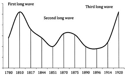
Fig. 1a. Long waves cycles illustration
Source: authors' approximation based on Kondratieff (1935).
One of the first to catch on the logic was Schumpeter (1939) who pointed out the distinction between short (Kitchin cycles of 3–4 years), medium (Juglar cycles of 9–10 years),[1] and long (Kondratieff cycles of 54–60 years) cycles in his analysis of economic development. We discuss some of them below.
As to mechanisms, Kondratieff already pointed to a large-scale accumulation of innovative activity, that is inventions and processes modifications that required fifty or more years before complete insertion, absorption in the production method. The role of innovation, implied in Kondratieff's analysis, is captured by the internal dynamic tendencies described in detail in Schumpeter's The Theory of Economic Development (Schumpeter 2007 [1934]). In turn, Garvy (1943) subjects Kondratieff's proposition to sharp criticism from positions of Soviet economists and from the point of view of Western economics. Paradoxically, in either case the conclusion appears to be that Kondratieff was too hasty in assigning the term ‘cycle’ to his propositions, as those do not correspond to the internal evolutionary dynamics following some mechanism of cycles.
There was a difference however in the Western economists' views and their contemporary Soviet counterparts. From the Western economist point of view, articulated by Garvy (Ibid.), there was no sufficient statistical evidence to warrant any regularity, that is cyclicality, to Kondratieff's analysis. The Soviet economists writing around the time of Kondratieff's original publications and shortly after (e.g., Studensky, Oparin, Pervushin, Bogdanov, Sukhanov and others, see Garvy 1943 for concise discussion and references) rejected the term ‘cycle’ in reference to the capitalist production mode since that implied some type of capitalist system's perpetuity. At the time that was in direct opposition with the socialist beliefs of gradual phasing out of the capitalist economy into its next logical stage of socialism, as was implied by then dominant interpretation of Marx's Capital (2003 [1867]). These beliefs in rapid phased successions picked up from simplistic interpretations would feed into initial enthusiasm around shock therapy reforms in post-socialist economies in the early 1990s (Gevorkyan 2011).
Recently, researchers working within Kondratieff's original methodological scope have attempted to extend their analysis across the twentieth century with focus on predictive capabilities of such work into the nearest future. Some find the ongoing economic deterioration in the world economy fitting calculations of the Fifth Long Wave of the Kondratieff cycle (e.g., Korotayev and Tsirel 2010; Kondratieff 2002; Akaev 2009; and others), some of them using spectral analysis. A re-validation of the very four exogenous shocks (technology, wars, shifts in boundaries, and value of gold) so carefully documented and refuted by Kondratieff himself took place in some of those papers. Exogenous shocks are surely important ‘occurrences’, yet, the internal dynamics in the evolution of economic relationships over a long time period and staging economic development must be considered as well. We address this in further detail below, using more modern empirical methods.
2.2. Kuznets' novel analysis of development
Simon Kuznets received the Nobel Prize in Economics in 1971 for his empirical analysis of economic growth, where he identified a new era of ‘modern economic growth’. Like Kondratieff, Kuznets relied on empirical analysis and statistical data in his pioneering research. Absorbing his findings on historical development of the industrial nations with initially abstract categories of the national income decomposition, Kuznets developed a concept of long swings, though disputed, now referred to as Kuznets cycles or Kuznets swings (e.g., Korotayev and Tsirel 2010).
The Kuznets swings' period is ranged between 15–25 years and initially connected by Kuznets with demographic cycles. In that analysis, the economist observed and quantified the cyclicality of production and prices, linking with immigrant population flows and construction cycles. Researchers have attempted to connect these cycles with investments in fixed capital or infrastructure investments (see Ibid. for literature review). Focusing on developed economies of North America and Western Europe, Kuznets computed national income from late 1860 forward with structural breakdowns by industry and final products. He also provided measures of income distribution between rich and poor population groups.
Kuznets unveiled the deficiency of constrained theoretical work built on simplified assumptions. He was critical of capital and labor as the sole factors sufficient for economic growth. Instead analysis must encompass information on technology, population and labor force skills, trade, markets, and government structure. Kuznets carried his analysis further in developing measures of national income through categories of consumption, savings, and investment (e.g., Kuznets 1949, 1937, 1934, etc.), eventually leading to a system of national income accounting.
It should also be noted that while working on the problem of income inequality, Kuznets was one of the first to look at economic growth measurements in the developing world (e.g., Kuznets 1971, 1966, and 1955). His well-known inverted U-shaped curve measuring inequality on the y-axis and economic development, expressed as change in GNP on the x-axis was an intellectual breakthrough of the time (see Fig. 1b). The conclusion is that while the economy remains in agricultural stage income inequality among different groups within the economy is low. As the national economy embarks on the process of industrialization inequality rises over time, then it falls again.
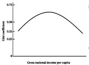
Fig. 1b. Kuznets curve
This describes the experience of developed economies in Western Europe and North America, that is the initial phases of industrialization cause sharp rises in inequality. Upon reaching a critical saturation point, inequality subsides while economic growth continues. This happens through the emergence of a ‘middle class’, improved education facilities, health care, and governance. It is interesting to note that further structural change and the shifting of resources to services and the financial sector, may increase inequality again, as, for example, is seen in the U.S. economy since the 1980s. It may be argued that this somewhat correlates to a popular analysis in development economics on the transition mechanisms from traditional to modern industrial sectors.
A variant of the Kuznets curve is also utilized in the analysis of environmental problems. This application suggests an immediate deterioration in air quality and intensification of environmental problems at the initial industrializing stages until spreading affluence and emergence of middle class introduces legislative and other controls on hazardous production (WB 1992; Grossman and Krueger 1995 and more recently Stern 2004). Elsewhere, these implied predictions of fading inequality offered a strong intellectual foundation for the mentioned reforms of the early 1990s in Eastern Europe and the former Soviet Union (Gevorkyan 2011). In studies of sequencing of market liberalization reforms and limitations of the state in the economy there were omitted the negative externalities of shock therapy policies. Yet, in the early 1990s, the promise of immediate market reforms and potential access to greater income opportunities did not materialize at the height of the reforms. In fact, income inequality problems still remain relevant and critical on policymakers' agendas two decades since the ‘transition’. The absence of the universal tendency of declining income inequality raises a question of how one measures economic development and what time-frame to consider is ‘sufficient’ to measure the rise of ‘welfare’ over time.
Finally, Kuznets (1973) brings up six key characteristics of modern economic growth, based on methodology consistent with national income accounting and historical analysis of economic development: 1) increase in per capita growth and population in developed economies; 2) increasing productivity rates; 3) increasing rate of structural transformation; 4) rising urbanization and secularization; 5) spread of technology and infrastructure improvements (communications); 6) limits to wide-scale spread of economic growth and benefits. Therefore despite seeming improvements, Kuznets noted persistence of disproportionate economic growth worldwide and apparently some broader measures of welfare.
Broadly speaking, such persistence of long wave-like tendencies on a global scale, a feature of contemporary industrial and financial globalization, supports the concept of redefined fundamental uncertainty (Gevorkyan and Gevorkyan 2012). Here the uncertainty of the direction, length, and capability of the post-great recession's potential recovery remains unclear. The lesser-developed economies (aka emerging markets) are worst affected in such circumstances, as the speculative foreign capital exits and industrial capacity remains inadequate on global competitive scale with absent technological advance.
Common between the work of both Kondratieff and Kuznets was the motivation to define the mechanisms of economic growth and development, and systematize core tendencies driving the transformational momentum. That in turn connects directly to the earlier discussion on cyclicality in development.
3. Time Scales and Mechanisms of Economic Cycles
As mentioned, the work of Kondratieff and Kuznets fostered a systematic approach to modern understanding of long economic swings. Numerous authors have further proposed not only different mechanisms underlying cycles but also cycles on different time scales. An early theory of cycles was put forward by Robert Owen in 1817, who stressed wealth inequality and poverty, originating in industrialization, yielding under-consumption as a reason for economic crises. Sismondi, in the middle of the 19th century took a similar view and developed a theory of periodic crises due to under-consumption. This led to the discussion of the ‘general glut’ theory of the 19th century, which Marx and other classical economists also extensively contributed to.
More specifically, a mechanism of cycles on a shorter times scale, of 8–10 years duration, was developed by Juglar (Juglar cycles), resulting, as he saw it, from the waves in fixed investment. Later, Kitchin, in the 1920s, introduced an inventory cycle of 3–5 years. Later an important contribution was made by Schumpeter (1939), who referred to the ‘bunching’ of innovations and their diffusion as a cause for long waves in economic activity.
Roughly at the same time, Samuelson (1939), influenced by the Spiethof accelerator and the Keynesian multiplier principle, developed the first mathematically-oriented cycle theory using difference equations.[2] Others, such as Rostow (1975), had proposed the theory of stages of growth. Simultaneous with Samuelson, Kalecki (1937) developed his theory of investment implementation cycles where he saw significant delays between investment decisions and investment implementations, formally introducing differential delay systems as tool for studying cycles.
Kaldor (1940), rooted in Keynesian theory, developed his famous nonlinear investment-saving cycles, which took into account aggregate demand. Later, Goodwin (1967) proposed a model of growth cycles, which took into account classical growth theory, but was based on unemployment-wage share dynamics, since the overall growth rate, as well as productivity growth, are kept constant in the long run. We will first discuss cycle theories on a longer time scale and then move to the Goodwin and Keynes-Kaldor cycles. We also briefly include a discussion of Kalecki's cycle theory (1971) and how it might relate to Kondratieff.
3.1. The Kondratieff long swings
The above review raises a few critical questions that need proper evaluation. For example, it is difficult to detect clear mechanisms in the Kondratieff cycles (e.g., as sketched in Fig. 1a above). If anything is working here as a mechanism, it must be some exhaustion of endogenous and exogenous factors: in the long upswing prices are rising, interest rates rise and wages rise, raw materials and non-renewable resources may be exhausted, causing to drive up prices and wages. New technologies are discovered in periods of long down swings, which come to be used in a new upswing. New resources are discovered, such as iron ore, coal, gold and other metals, which Kondratieff argues to be endogenously expanded through new discoveries but both technology and resources will finally be exhausted too: resource and product prices rise, deposits at saving banks rise, but also interest rates and wages rise and a downturn begins. There is a struggle for markets and resources. New countries are opened up. There are market limits, such export limits, which restrict further expansions, as Kondratieff data on French exports show. Then, in the long downswing, prices fall, wages fall, interest rates fall, plenty of resources and unused production capacity push prices down, and unemployment reduces wages. Overall, there are some mechanisms indicated in Kondratieff, but not specifically modeled.
3.2. The Kuznets long swings
Further, Kuznets theory of development and fluctuations can be seen as an interesting intersection of two traditions in the economics of his time. On the one hand, he was interested in cyclical movements in numerous time series data, such as volume of all types of production and prices, seasonal and secular movements in industry income and national income and its components, long swings in economic activities, and business cycle analysis. On the other hand, he saw development as a time irreversible process of industry and national income development, which evolves in stages of economic growth, with plenty of structural changes. Each stage may have its particular saving rate, consumption patterns, unevenness and disequilibrium as well as income inequality. As described above, inequality first rises with industrialization and later declines. Kuznets conceptual framework can be seen as a mixture of cycle theories, referring to the accelerator principle for infrastructure investments, and a theory of stages of economic growth that were similar to those pursued by Rostow (1975). A similar view on stages of growth, that taken by Kuznets and Rostow, is also pursued by Greiner, Semmler and Gong (2005). Overall, Kuznets was ambiguous whether there are regular mechanisms generating cycles. He conjectured that cycles may be in the economic data solely as a result of certain historical ‘occurrences’.
3.3. The Schumpeter innovation cycles
Schumpeter's concept of competition deviates from the neoclassical conception in some essential aspects. First, competition is not limited to price or quantity adjustments. It is described as an evolutionary process, as a process of ‘creative destruction’. The engines of this development are capitalist enterprises. ‘Capitalism, then, is by nature a form or method of economic change and not only never is but never can be stationary ... The fundamental impulse that sets and keeps the capitalist engine in motion comes from the new consumer's goods, the new methods of production or transportation, the new markets, the new forms of industrial organization that capitalist enterprise creates’ (Schumpeter 1970: 83). The incentives for developing these types of technical change originate in transient surplus profits. What is taken as given in neoclassical general equilibrium analysis as parametric data, when the price and quantity adjustments occur is the explicandum in Schumpeter: process innovation, product innovation, new forms of organization of the firm and new forms of financial control.
Second, Schumpeter stresses that competition is not necessarily an equilibrating force. When referring to the existence of entrepreneurial firms and their rivalry, Schumpeter maintains that ‘there is in fact no determinate equilibrium at all and the possibility presents itself that there may be an endless sequence of moves and counter-moves, an indefinite state of warfare between firms’ (Ibid.: 79). Moreover, competition as an evolutionary process takes place through time, in discrete steps. For example, he writes, ‘Now the first thing we discover in working out the propositions that thus relate quantities belonging to different points in time is the fact that, once equilibrium has been destroyed by some disturbances, the process of establishing a new one is not so sure and prompt and economical as the old theory of perfect competition made it out to be, and the possibility that the very struggle for adjustment might lead such system farther away instead of nearer to a new equilibrium. This will happen in most cases unless the disturbance is small’ (Ibid.: 103). Indeed, in Schumpeter it is the product and process innovation, undertaken by the entrepreneur, which brings the economic system out of equilibrium, resulting in long waves and business cycles. Moreover, he even does not seem to be very interested in a theory of centers of gravitation for market forces as developed by the classical economists.
Third, in Schumpeter, competition is an evolutionary process, one of rivalry between firms motivated by the search for surplus profit. He calls this surplus profit the transient ‘monopoly profit’ of new processes and new products, ‘Thus, it is true that there is or may be an element of genuine monopoly gain in those entrepreneurial profits which are the prizes offered by capitalist society to the successful innovator. But the quantitative importance of that element, its volatile nature and its function in the process in which it emerges put it in a class by itself’ (Ibid.: 102). ‘The transient surplus profit does not appear as deviation from the perfectly competitive state of the economy and as a waste in the allocation of resources, but as a reward for the innovator and a gain for the capitalist society. On the contrary, the perfectly competitive economy, where every market agent behaves in the same way under the condition of parametrically given external conditions seems to imply a waste of resources ... working in the conditions of capitalist evolution, the perfect competitive arrangement displays wastes of its own. The firm of the type that is compatible with perfect competition is in many cases inferior in internal, especially technological, efficiency. If it is, then it wastes opportunities’ (Schumpeter 1970: 106). Thus, in Schumpeter's view, the entrepreneurial firms are powerful engines of progress and ‘in particular of the long-run expansion of total output’ (Ibid.).
Following Schumpeter's footsteps, the literature after Schumpeter has distinguished between radical and incremental innovation. The major waves of radical innovations, which were followed by the diffusion of this new technology and incremental innovations are.[3]
· The water-powered mechanization of the industry of the 18th and early 19th century;
· The steam-powered mechanization of the industry and transport of the middle of the 19th century (rail ways, steam engines, machine tools);
· The electrification of industry, transport and homes at the end of the 19th century;
· Motorization of industrial production, transport, civil economy and the war machinery (from ~1914 onward);
· Computerization and information technology from the 1960s and 1970s onward.
According to Schumpeter's oriented long wave theories, each of those radical innovations did not only create long waves in economic development, but each of those long waves were driven by different technology, originated in different countries and then diffused world wide.
3.4. The Samuelson accelerator-multiplier cycles
A model of medium-time scale is the one created by Samuelson (1939). The basic construction is as follows: consumer spending (via increased sales by firms) accelerates investment; output changes results in income changes through the multiplier, which, in turn, again stimulates sales, that is consumer spending.
The multiplier-accelerator model of Samuelson (Ibid.) can produce cycles. Take Сt = consumption, It = investment, Yt = income, C0 = autonomous consumption, I0 = autonomous investment, and G = C0 + I0; I = S = sY, therefore the multiplier is: ![]() Use:
Use:
Ct = C0 + αYt – 1, (1)
It = I0 + β (Yt – 1 – Yt – 1), (2)
Yt = Сt + It . (3)
Substituting (1) and (2) into (3) gives
Yt = С0 + αYt – 1 + I0 + βYt – 1 – βYt – 2,
G = C0 + I0,
Yt = G + (α + β) Yt – 1 – βYt – 2.
The standard form of a second order linear difference equation is:
Yt – (α – β) Yt – 1 + βYt – 2 = G, (4)
which is stable or unstable depending on the size of ?. Moreover, one can have contracting or expanding cycles depending on whether there exist imaginary parts of the eigenvalues (see Figs 2a – 2d).
When we replace income by profit flows Rt, one can turn the above into a kind of Kalecki model such as: It + 1 = A + αRt + b(Rt – Rt – 1). If one writes for spRt = It, ![]() , we get a similar second order difference equation:
, we get a similar second order difference equation:
![]() , (5)
, (5)
which again can be stable or unstable and it can produce unidirectional change or oscillations. The Kalecki model is further studied in Sub-section 3.7.
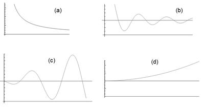
Figs 2a – 2d. Stable and unstable development and oscillations
3.5. The Goodwin growth and income distribution cycles
Other types of cycles that have been discussed, particularly in the Post War II period, where Goodwin's growth cycle theory that postulates an interaction of employment and wage share. It looked like a business cycle model when it was first proposed but, in fact, empirically it seems to operate also on a medium time scale.[4]
Goodwin (1967) postulates cycles driven by growth and income distribution. Low growth, generated by low profits and investment, generates unemployment, which in turn limits wage growth as compared to productivity. This gives rise to lowering the wage share: low wage share means high profit share and slowly rising investment, which reaches a turning point as employment and wage growth make the wage share rising and the profit share falling. By utilizing nonlinear differential equations, originally developed by Lotka and Volterra for the models of interacting populations, we can rewrite the Goodwin model of wage-employment dynamics as follows:
![]() ,
,
or as
 ,
,
where ![]() represents the time rate of change of the ratio of the employed to the total labor force and
represents the time rate of change of the ratio of the employed to the total labor force and ![]() is the change of the wage share. Both variables depend on the level of х and the constants a, b, c, d > 0. The coefficient, a, denotes the trend of employment if all income is reinvested (y = 0) and d is the fall in real wage if (x = 0). The symbol by denotes the influence of the wage share on the employment ratio, and cx the positive influence of employment on the wage share. Due to this interaction of the variables the employment ratio is prevented from rising and the wage share from falling without limits.
is the change of the wage share. Both variables depend on the level of х and the constants a, b, c, d > 0. The coefficient, a, denotes the trend of employment if all income is reinvested (y = 0) and d is the fall in real wage if (x = 0). The symbol by denotes the influence of the wage share on the employment ratio, and cx the positive influence of employment on the wage share. Due to this interaction of the variables the employment ratio is prevented from rising and the wage share from falling without limits.
For a growth model with trends as represented by Goodwin, the coefficients can be interpreted as follows: a = b – (m + n) where b is the output/capital ratio (Y/K), m is the growth rate of productivity and n is the growth rate of the labor force. All of those are taken as constants. Assuming a linearized wage function (for instance, ![]() and with m the growth rate of productivity as before, we obtain for the growth rate of the wage share the term
and with m the growth rate of productivity as before, we obtain for the growth rate of the wage share the term ![]() with m = d – e. Thus, the second pair of differential equations can be written as:
with m = d – e. Thus, the second pair of differential equations can be written as:
![]()
![]()
which is indeed equivalent to the first equation of the (above) system, except that it is written in terms of growth rates. The core of the last system shows that the change of the employment ratio depends on the profit share (1 – y) and that the change of the wage share depends on the employment ratio. This form has been used to explain the fluctuation of the employment ratio and the fluctuation of the industrial reserve army in Marx (Marx 2003 [1867]: ch. 23; see Goodwin 1967). The basic structure of this model represents the interacting variables of the employment ratio and wage share as dynamically connected.
The last system has two equilibria: (0, 0) and ![]() . The linear approximation of the system is with ξ1, ξ2 as small deviations from the equilibrium values
. The linear approximation of the system is with ξ1, ξ2 as small deviations from the equilibrium values
![]() .
.
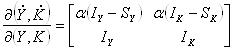
The calculation of the Jacobian for the first linear approximation gives for the equilibrium ![]()
The real parts of the eigenvalues are zero and the linear approximation of the equilibrium point represents the dynamical structure of a center (Hirsch and Smale 1974: 258). With real parts of the eigenvalues zero, the linear approximation of the system through the Jacobian does not allow conclusions regarding the behavior of the dynamical system in the neighborhood of the equilibrium. Yet, as can be shown, by constructing a Liapunov function for the above system, which is constant in motion and hence has time derivatives ![]() the wage share-employment dynamics results in closed solution curves (Ibid.; Flaschel and Semmler 1987).
the wage share-employment dynamics results in closed solution curves (Ibid.; Flaschel and Semmler 1987).
The closed trajectories of the system are, however, only closed curves and the wage share-employment dynamics does not allow for persistent cycles, such as limit cycles (Hirsch and Smale 1974: 262; Flaschel 1984). In addition (see Flaschel and Semmler 1987), the dynamical system is structurally unstable, since small perturbations can lead to additional interaction of the variables (J11 or J22 can become nonzero). This leads to a qualitatively different dynamical behavior of the system, hence it can become totally stable or unstable. Under certain conditions the above system can also become globally asymptotically stable. This can occur if the conditions for Olech's theorem are fulfilled (see Flaschel 1984).
Equivalent results are obtained when in place of a linear wage function a nonlinear wage function is substituted in the system (see Velupillai 1979). The wage share-employment dynamics worked out originally by Goodwin for a model of cyclical growth and then applied by him to explain an endogenously created unemployment of labor depict a growing economy, whereas often models of nonlinear oscillations refer only to a stationary economy.
Since the change of the wage share and the change of labor market institutions such as bargaining and other protective legislature are slow, this model of economic cycles, however, does not really model business cycles but rather medium run cycles. On the other hand, for a theory of longer cycles the dynamical interaction of other important variables over time (such as waves of innovations, changes of capital/output ratio, productivity, relative prices and interest rates) as well as demand factors are neglected.
3.6. The Keynes–Kaldor demand driven cycles
The demand factors are considered in the next section presented here. The Keynes–Kaldor model seems to operate on a shorter time scale. It essentially refers to the role of demand, defined by the relation of investment and savings. In his article, Kaldor (1940) proposed such a shorter scale cycle model, a nonlinear model of business cycles, which after that has been reformulated in the light of mathematical advances in the theory of nonlinear oscillations, which take into account demand changes (Kaldor 1940, 1971; Chang and Smyth 1971; Semmler 1986).
Kaldor relies on a geometric presentation of a business cycle model which depends on a nonlinear relation between income changes and capital stock changes and which seems to generate self-sustained cycles without rigid specifications for the coefficients, time lags and initial shocks. The geometric presentation of his model of persistent business cycles due to the dynamic interaction between income changes and accumulation and dissolution of capital indeed also includes the possibility of limit cycles, that is asymptotically stable cycles regardless of the initial shocks and time lags.
His ideas are also formulated for a stationary economic system and can be represented by nonlinear differential equations in the following way (Chang and Smyth 1971):
![]()
where α is a reaction coefficient, ![]() the rate of change of income,
the rate of change of income, ![]() the rate of change of the capital stock, I = investment and S = saving as functions of the level of income and capital stock. According to the assumptions underlying the model, there is a unique singular point (Ibid.: 40). This type of Keynesian–Kaldorian model can give rise to persistent cycles (see Semmler 1986), it does not model the specific role of growth and income distribution, as Goodwin has stressed. Yet it stresses the role of endogenously changing demand. The linear approximation is:
the rate of change of the capital stock, I = investment and S = saving as functions of the level of income and capital stock. According to the assumptions underlying the model, there is a unique singular point (Ibid.: 40). This type of Keynesian–Kaldorian model can give rise to persistent cycles (see Semmler 1986), it does not model the specific role of growth and income distribution, as Goodwin has stressed. Yet it stresses the role of endogenously changing demand. The linear approximation is:
![]() ,
,
where the Jacobian is
 ,
,
where ![]() since
since ![]() and
and ![]() (Chang and Smyth 1971: 41). The determinant is
(Chang and Smyth 1971: 41). The determinant is ![]() which is positive because for the existence of a unique singular point it is assumed that
which is positive because for the existence of a unique singular point it is assumed that ![]() . The element,
. The element,![]() , is always negative. The linear approximation with the Jacobian represents at its core the investment-income dynamics according to which the change of income depends negatively on the level of the capital stock
, is always negative. The linear approximation with the Jacobian represents at its core the investment-income dynamics according to which the change of income depends negatively on the level of the capital stock ![]() and the change of capital stock depends positively on the level of income
and the change of capital stock depends positively on the level of income ![]() but there is a negative feedback effect from the level of capital stock to the change of capital stock and an ambiguous feedback effect from the level of income to the change of income
but there is a negative feedback effect from the level of capital stock to the change of capital stock and an ambiguous feedback effect from the level of income to the change of income ![]() . This will be explained subsequently.
. This will be explained subsequently.
Analyzing the singular point one can conclude that the equilibrium is a focus or a node and that the equilibrium is stable or unstable accordingly as ![]() This singular point also allows for a limit cycle, since the necessary condition for a limit cycle is that the dynamic system has an index of a closed orbit, equal to 1 (Minorsky 1962: 79). This excludes a saddle point as a singular point (see Ibid.: 77). Moreover, the most interesting point in this dynamic system is the ambiguous element
This singular point also allows for a limit cycle, since the necessary condition for a limit cycle is that the dynamic system has an index of a closed orbit, equal to 1 (Minorsky 1962: 79). This excludes a saddle point as a singular point (see Ibid.: 77). Moreover, the most interesting point in this dynamic system is the ambiguous element ![]() . According to Kaldor's graphical presentation, it is assumed (see Kaldor 1940: 184) that
. According to Kaldor's graphical presentation, it is assumed (see Kaldor 1940: 184) that
(1) ![]() for a normal level of income;
for a normal level of income;
(2) ![]() for abnormally high or abnormal lowly levels of income; and
for abnormally high or abnormal lowly levels of income; and
(3) the stationary state equilibrium has a normal level of income.

Fig. 3. Kaldor graph on nonlinear investment and saving functions
This might be illustrated by Fig. 3 with Y being the level of output, which shows that the normal level of Y is unstable and the extreme values of Y are stable. Mathematically this means that the trace ![]() changes signs during cycles. This is the negative criterion of Bendixson (Minorsky 1962: 82) for limit cycles, that is if the trace
changes signs during cycles. This is the negative criterion of Bendixson (Minorsky 1962: 82) for limit cycles, that is if the trace ![]() does not change signs, persistent cycles – limit cycles – cannot exist (see also Guckenheimer and Holms 1983: 44). As proven by Chang and Smyth (1971: section V), there indeed exists the possibility of stable cycles, limit cycles, under the assumption proposed by Kaldor.
does not change signs, persistent cycles – limit cycles – cannot exist (see also Guckenheimer and Holms 1983: 44). As proven by Chang and Smyth (1971: section V), there indeed exists the possibility of stable cycles, limit cycles, under the assumption proposed by Kaldor.
However, the three conditions as formulated above and originally formulated by Kaldor (1940: 1984) are not necessary for the existence of cycles. What is actually necessary for cycles is only that ![]() (i.e. that
(i.e. that ![]() switches signs) at some level of Y. Moreover, the singular point at the normal level of Y does not have to be unstable as a necessary condition for a limit cycle. The critical point can be stable (see Minorsky 1962: 75). In addition there also is the possibility that the system is globally asymptotically stable. This is the case if:
switches signs) at some level of Y. Moreover, the singular point at the normal level of Y does not have to be unstable as a necessary condition for a limit cycle. The critical point can be stable (see Minorsky 1962: 75). In addition there also is the possibility that the system is globally asymptotically stable. This is the case if: ![]() and (2)
and (2) ![]() everywhere.
everywhere.
The global asymptotic stability under these conditions follows from Olech's theorem (see Ito 1978: 312).
Evaluating Keynes–Kaldor's model of a demand driven business cycles one can say that Kaldor's formulation of an income-investment dynamics brought some advances regarding a theory of endogenously produced business cycles, especially formulations of the theory of cycles in terms of a theory of nonlinear oscillations (see also Kaldor 1971) one can extend this to include a formulation concerning the dynamics in employment and wage share which was originally more visible in classical models that referred to the profit-investment dynamics.
3.7. The Kalecki profit and investment cycles
To draw some similarities to the Kondratieff long wave theory, we can follow Kalecki (1971) and replace the income, Y, by profit flows П[5] and allow for ![]() to change its sign during the cycle. In some sense the role of profit, wages and income distribution – as in the Goodwin model – can be allowed to come in here.
to change its sign during the cycle. In some sense the role of profit, wages and income distribution – as in the Goodwin model – can be allowed to come in here.
In general it could be assumed that:
(Case 1) ![]() for profit income in an interval such as П1 < П < П2 (see Fig. 4). This may be due to a previous decrease in capital stock, production and employment which entail low construction cost for plants, low material and resource cost and low wage costs (relative to productivity), high profits and low interest rates and easy access to credit. These factors then may give rise to an expectation of rising profits on investments.
for profit income in an interval such as П1 < П < П2 (see Fig. 4). This may be due to a previous decrease in capital stock, production and employment which entail low construction cost for plants, low material and resource cost and low wage costs (relative to productivity), high profits and low interest rates and easy access to credit. These factors then may give rise to an expectation of rising profits on investments.
On the other hand, in other regions we can have:
(Case 2) ![]() with two clarifying conditions:
with two clarifying conditions:
(a) for П > П2 due to capacity limits, rising construction cost for plants and rising material and wage cost (relative to productivity), exhaustion of exhaustible resources, rising interest rates and but falling actual and expected profits. Profits and expected profits may fall due to the rise of those costs and wages – that cannot be passed on – in the long upswing. This looks similar to a mechanism that Kondratieff has indicated to eventually occur in his long upswing (see Sections 2.1 and 3.1).
(b) for П < П1 in a recessionary or slow recovery period, where firms invest in financial funds instead of in real capital (Minsky 1983) but due to the economic conditions in a recessionary period, the rate of change of saving in response to falling profits tend to drop faster than the rate of change of investment. Wage share may have been rising previously, and profit share falling but here investment is still not dropping completely to zero. This resembles the Kondratieff scenario of a long downswing and recessionary or stagnation period.
Though the economic intuition appears the same in our above stylized business cycle dynamics and the Kondratieff long waves phases, the time scales are probably different ones: one is a shorter one and the other a longer one, but the mechanisms may be the same. Yet, for a longer time scale much of the economic structure and relationships are likely to change.
In the history of economic thought the change of sign for ![]() during the economic cycle was verbally anticipated by many writers on the study of capitalist dynamics (Kalecki 1971: 123; Kaldor 1940: 184) and can be regarded as essential for a theory of fluctuations in economic development. Mathematically
during the economic cycle was verbally anticipated by many writers on the study of capitalist dynamics (Kalecki 1971: 123; Kaldor 1940: 184) and can be regarded as essential for a theory of fluctuations in economic development. Mathematically ![]() must change signs in order to generate self-sustained cycles. If
must change signs in order to generate self-sustained cycles. If ![]() and
and ![]() were zero,
were zero, ![]() and
and ![]() alone would determine the profit-investment dynamics. There would only be structurally unstable harmonic oscillations. The negative signs of
alone would determine the profit-investment dynamics. There would only be structurally unstable harmonic oscillations. The negative signs of ![]() and
and ![]() exert a retarding influence on accumulation, and
exert a retarding influence on accumulation, and ![]() represents an accelerating force on capital accumulation, whereas
represents an accelerating force on capital accumulation, whereas ![]() exerts a retarding influence in the boom period and an accelerating impact on profit and accumulation in the later phase of the recession.
exerts a retarding influence in the boom period and an accelerating impact on profit and accumulation in the later phase of the recession.
Intuitively, the existence of self-sustained cycles can be seen in Fig. 4 from the fact that the trajectories of П(t) and К(t) are bounded in absolute values and the profit-investment dynamics follow certain directions in the plane. Roughly speaking, for large enough П(t), ![]() turns negative and for large enough К(t),
turns negative and for large enough К(t), ![]() turns negative and vice versa. Geometrically, this is illustrated by Fig. 4.
turns negative and vice versa. Geometrically, this is illustrated by Fig. 4.
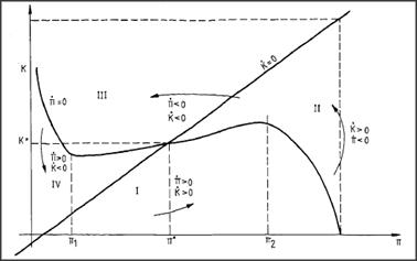
Fig. 4. Phase diagram
For ![]() we get the slope
we get the slope
![]() ,
,
and for ![]() the slope is
the slope is
![]() .
.
![]() Thus, in the plane of the Fig. 4 there are four quadrants. For reasons of simplicity we have assumed a linear investment function in Fig. 4. The system has a unique solution at П* and K* since the curve
Thus, in the plane of the Fig. 4 there are four quadrants. For reasons of simplicity we have assumed a linear investment function in Fig. 4. The system has a unique solution at П* and K* since the curve ![]() has a steeper slope than
has a steeper slope than ![]() when the latter is upward sloping in a certain region. This follows from the assumption in the model.[6] The determinant of the Jacobian of the dynamical system above is
when the latter is upward sloping in a certain region. This follows from the assumption in the model.[6] The determinant of the Jacobian of the dynamical system above is ![]() The singular point is a focus or a node and is stable or unstable accordingly as
The singular point is a focus or a node and is stable or unstable accordingly as ![]() < 0. A saddle is excluded, and the singular point has index 1 as necessary condition for a self-sustained cycle (Minorsky 1962: 176). (The singular point does not have to be unstable as Kaldor originally assumed; see Kaldor 1940: 182.) The existence of a self-sustained cycle follows intuitively from the analysis of the vector fields in the different regions, which correspond roughly to stages of economic cycles.[7]
< 0. A saddle is excluded, and the singular point has index 1 as necessary condition for a self-sustained cycle (Minorsky 1962: 176). (The singular point does not have to be unstable as Kaldor originally assumed; see Kaldor 1940: 182.) The existence of a self-sustained cycle follows intuitively from the analysis of the vector fields in the different regions, which correspond roughly to stages of economic cycles.[7]
For region I, which expresses the dynamics of a recovery period, К(t) is below the ![]() curve and П(t) is below the
curve and П(t) is below the ![]() curve; the decline in capital stock and its effect on profit (i.e. the effects of Cases 1 and 2) as well as other changes in economic conditions in a recessionary period will generate a positive rate of change of profit (since
curve; the decline in capital stock and its effect on profit (i.e. the effects of Cases 1 and 2) as well as other changes in economic conditions in a recessionary period will generate a positive rate of change of profit (since ![]() in region I, see also Case 1). Therefore, in region I we will find
in region I, see also Case 1). Therefore, in region I we will find ![]() and
and ![]()
The increase of profits and investments after a recessionary period will lead to rising К(t), but through the effect of Cases 1 and 2 (i.e. the negative effect of growth of capital stock on profits) the growth rate of II will become negative. Thus, in region II, indicating a boom period, we have ![]() and
and ![]() Hence, the arrows in Fig. 4, indicating the direction of the vector field of П and K, will start bending inward (see Case 2a which leads to
Hence, the arrows in Fig. 4, indicating the direction of the vector field of П and K, will start bending inward (see Case 2a which leads to ![]() ). With capital stock rising and
). With capital stock rising and ![]() due to a magnitude of capital stock greater than its stationary value K*, the capital stock must eventually decline (i.e. through the effect of Case 2). We also have
due to a magnitude of capital stock greater than its stationary value K*, the capital stock must eventually decline (i.e. through the effect of Case 2). We also have ![]() due to
due to ![]() at the beginning of a downswing period (capital may be accumulated more as money capital than as real capital).
at the beginning of a downswing period (capital may be accumulated more as money capital than as real capital).
In region III, indicating a downswing period, through the influence of ![]() on K(t), K(t) also starts declining; thus
on K(t), K(t) also starts declining; thus ![]() and
and ![]() Hence, for
Hence, for ![]() and
and ![]() the vector field is pointing inward. A decline of capital stock below K* in region IV, the recessionary period, however, eventually causes profits to rise. The recessionary period may slowly then turn into a recovery period, indicated by region I. This, of course, assumes again that eventually
the vector field is pointing inward. A decline of capital stock below K* in region IV, the recessionary period, however, eventually causes profits to rise. The recessionary period may slowly then turn into a recovery period, indicated by region I. This, of course, assumes again that eventually ![]() . The investment of financial funds turns into investment in real capital, thus investment out of profit tends to become greater than savings out of profit. The recessionary period (with wage increase below productivity, low material and capital cost, low interest rates and easy access to credit as well as a decline in capital stock and thus rising profit expectation[8] must have its impact on
. The investment of financial funds turns into investment in real capital, thus investment out of profit tends to become greater than savings out of profit. The recessionary period (with wage increase below productivity, low material and capital cost, low interest rates and easy access to credit as well as a decline in capital stock and thus rising profit expectation[8] must have its impact on![]() , for otherwise the recessionary period will endure.
, for otherwise the recessionary period will endure.
Therefore, under the economic conditions stated in Cases 1, 2a, and 2b the profit-investment dynamics creates its own cycles by which profit, investment and thus output and employment cannot exceed certain boundaries. The dynamic system is self-correcting and fluctuates within limits: for large enough K(t) is ![]() and for large enough П(t) is
and for large enough П(t) is ![]() . A similar argument holds for small enough K(t) and П(t). Thus, whereas the system with Cases 1 and 2 becomes stable at its outer boundaries (indicated by the negative sign of
. A similar argument holds for small enough K(t) and П(t). Thus, whereas the system with Cases 1 and 2 becomes stable at its outer boundaries (indicated by the negative sign of ![]() ), it cannot converge towards equilibrium, since the equilibrium is unstable (indicated by the positive sign of
), it cannot converge towards equilibrium, since the equilibrium is unstable (indicated by the positive sign of ![]() ). Therefore, the dynamics of the system will result in cycles (see Semmler 1986). These self-sustained cycles, resulting from the profit-investment dynamics, can be regarded as close to classical dynamics and conceptions and the original Kalecki model and reflects to a certain extent also the dynamics of output, income, resource cost, price level, wage and bank deposit and interest rate dynamics of the Kondratieff long wave theory. Though for such a cycle on long time scale many structural changes may occur that could significantly change the mechanisms and economic relationship over the cycle.
). Therefore, the dynamics of the system will result in cycles (see Semmler 1986). These self-sustained cycles, resulting from the profit-investment dynamics, can be regarded as close to classical dynamics and conceptions and the original Kalecki model and reflects to a certain extent also the dynamics of output, income, resource cost, price level, wage and bank deposit and interest rate dynamics of the Kondratieff long wave theory. Though for such a cycle on long time scale many structural changes may occur that could significantly change the mechanisms and economic relationship over the cycle.
4. The Minsky Financially Driven Basic Cycle and Super-Cycle
Next we discuss a Minsky long cycle: a financially-based approach to the long wave theory. Long cycles have historically been interpreted as an interaction of real forces with cost and prices. Kondratieff cycles emphasize secular changes in production and prices; Kuznets cycles are associated with economic development and infrastructure accumulation; Schumpeterian cycles are the result of waves of technological innovation; while Goodwin cycles are based on changes in the functional distribution of income arising from changed bargaining power conditions in a period of high growth rates and Keynesian theories express demand factors.
The work of Hyman Minsky provides an explicitly financially driven theory of business cycles. Minsky's own writings were largely devoted to exposition of a short-run cycle and a very long-run analysis of stages of development of capitalism. The short-run analysis is illustrated in two articles (Minsky 1957, 1959) that present a financially driven model of the business cycle based on the multiplier-accelerator mechanism with floors and ceilings. A later formalization is the Delli Gatti et al.'s work (1994) in which the underlying dynamic mechanism is increasing leveraging of profit flows, which roughly captures Minsky's (1992a) hedge-speculative-Ponzi finance transition dynamic that is at the heart of his famous financial instability hypothesis. The very long-run analysis of stages of capitalism's development is illustrated in Minsky's (1992b) essay on ‘Schumpeter and Finance’. These stages of development perspective have been further elaborated by Whalen (1999) and Wray (2009).
Recently, Palley (2010, 2011) has argued Minsky's (1992a) financial instability hypothesis also involves a theory of long cycles. This long cycle explains why financial capitalism is prone to periodic crises and it provides a financially grounded approach to understanding long wave economics.
A long cycles perspective provides a middle ground between short cycle analysis and stages of development analysis. Such a perspective was substantially developed by Minsky in a paper co-authored with Piero Ferri (Ferri and Minsky 1992). However, unfortunately, Minsky entirely omitted it in his essay (Minsky 1992a) summarizing his financial instability hypothesis, leaving the relation between the short and long cycle undeveloped.
Minsky's financial instability hypothesis maintains that capitalist financial systems have an inbuilt proclivity to financial instability that tends to emerge in periods of economic tranquility. Minsky's framework is one of evolutionary instability and it can be thought of as resting on two different cyclical processes (Palley 2010, 2011). The first is a short cycle and can be labeled the ‘Minsky basic cycle’. The second is a long cycle that can be labeled the ‘Minsky super cycle’.
The Minsky basic cycle has been the dominant focus of interest among those (mostly Post Keynesians) who have sought to incorporate Minsky's ideas into macroeconomics and it provides an explanation of the standard business cycle. The basic cycle is driven by evolving patterns of financing arrangements and it captures the phenomenon of emerging financial fragility in business and household balance sheets. The cycle (see Fig. 5) begins with ‘hedge finance’ when borrowers' expected revenues are sufficient to repay interest and loan principal. It then passes on to ‘speculative finance’ when revenues only cover interest, and the cycle ends with ‘Ponzi finance’ when borrowers' revenues are insufficient to cover interest payments and they rely on capital gains to meet their obligations.
Fig. 5. Minsky financing practices
The Minsky basic cycle embodies a psychologically based theory of the business cycle. Agents become progressively more optimistic in tranquil periods, which manifest itself in increasingly optimistic valuations of assets and associated actual and expected revenue streams, and willingness to take on increasing risk in belief that the good times are here forever. This optimistic psychology affects credit volume via the behavior of both borrowers and lenders – not just one side of the market. That is critical because it means market discipline becomes progressively diminished. Leveraging is increased but the usual text book scenario of corporate finance, whereby higher leverage results in higher risk premia, is not visible in the cost of credit. Instead, credit remains cheap and plentiful because of these psychological developments.
Our empirical analysis in Section 5.4 illustrates this credit dynamic for the recent long financial cycle beginning in the 1990s. Initially, it was a real cycle driven by information technology (IT). This IT bubble burst around 2000/2001. However, expansion resumed, owing to Minsky's financial cycle of over-optimism, high leverage, underestimation of risk, and expansion of new financial practices. The data show a high degree of leveraging during this period, an optimistic view of profit expectations, low risk premia, low credit spreads, and few credit constraints. Thus, contrary to corporate finance textbooks, the market generated high leveraging with low risk premia.
This process of increasing optimism, rising credit expansion and low risk perception is evident in the tendency of business cycle expansions to foster talking about the ‘death of the business cycle’. In the USA, the 1990s experienced much ‘talk’ of a ‘new economy’ which was supposed to have killed the business cycle by inaugurating a period of permanently accelerated productivity growth. That was followed, in the 2000s, by ‘talk’ of the ‘Great Moderation’ which claimed central banks had tamed the business cycle through improved monetary policy based on improved theoretical understanding of the economy. It is precisely this ‘talk’ which provides prima facie evidence of the operation of the basic Minsky cycle.
Moreover, not only does the increasing optimism driving the basic cycle afflict borrowers and lenders, it also afflicts regulators and policymakers. That means market discipline is weakened both internally (weakened lender discipline) and externally (weakened regulator and policymaker discipline). For instance, Federal Reserve Chairman Ben Bernanke (2004) openly declared himself a believer in the Great Moderation hypothesis.
The basic Minsky cycle is present in every business cycle and explains the observed tendency toward increased leverage and increased balance sheet fragility over the course of standard business cycles. However, it is complemented by the Minsky super cycle, that works over a longer time scale of several business cycles. This long-cycle rests on a process that transforms business institutions, decision-making conventions, and the structures of market governance including regulation. Minsky (Ferri and Minsky 1992) labeled these structures ‘thwarting institutions’ because they are critical to holding at bay the intrinsic instability of capitalist economies. The process of erosion and transformation of thwarting institutions takes several basic cycles, creating a long phase cycle relative to the basic cycle.
The basic cycle and long-cycle operate simultaneously so that the process of institutional erosion and transformation continues during each basic cycle. However, the economy only undergoes a full-blown financial crisis that threatens its survivability when the long-cycle has had time to erode the economy's thwarting institutions. This explains why full-scale financial crises are relatively rare. In-between these crises, the economy experiences more limited financial boom-bust cycles. Once the economy is in a full-scale crisis, it enters a period of renewal characterized by thwarting institutions, with new laws and regulations established and governing institutions empowered. That happened during the Great Depression of the 1930s and it is happening again, following the financial crisis of 2008.
Analytically, the Minsky long-cycle can be thought of as allowing more and more financial risk into the system via the twin developments of ‘regulatory relaxation’ and ‘increased risk taking’. These developments increase both the supply of and demand for risk.
The process of regulatory relaxation has three dimensions. One dimension is regulatory capture whereby the institutions intended to regulate and reduce excessive risk-taking are captured and weakened. Over the past twenty-five years, this process has been evident in Wall Street's stepped up lobbying efforts and the establishment of a revolving door between Wall Street and regulatory agencies such as the Securities and Exchange Commission, the Federal Reserve, and the Treasury Department. A second dimension is regulatory relapse. Regulators are members of and participants in society, and like investors they are also subject to memory loss and reinterpretation of history. Consequently, they too forget the lessons of the past and buy into rhetoric regarding the death of the business cycle. The result is willingness to weaken regulation on grounds that things are changed and regulation is no longer needed. These actions are supported by ideological developments that justify such actions. That is where economists have been influential through their theories about the ‘Great Moderation’ and the viability of self-regulation. A third dimension is regulatory escape whereby the supply of risk is increased through financial innovation. Thus, innovation generates new financial products and practices that escape the regulatory net because they did not exist when current regulations were written and are therefore not covered.
The processes of regulatory capture, regulatory relaxation, and regulatory escape are accompanied by increased risk taken by borrowers. First, financial innovation provides new products that allow investors to take more risky financial positions and borrowers to borrow more. Recent examples of this include home equity loans and mortgages that are structured with initial low ‘teaser’ interest rates that later jump to a higher rate. Second, market participants are also subject to gradual memory loss that increases their willingness to take on risk. Thus, the passage of time contributes to forgetting of earlier financial crisis, which fosters new willingness to take on risk. The 1930s generation was cautious about buying stock in light of the experiences of the financial crash of 1929 and the Great Depression, but baby boomers became keen stock investors. The Depression generation's reluctance to buy stock explains the emergence of the equity premium, while the baby boomer's love affair with stocks explains its gradual disappearance.
Changing taste for risk is also evident in cultural developments. One example of this is the development of the ‘greed is good’ culture epitomized by the fictional character Gordon Gecko in the movie Wall Street. Other examples are the emergence of investing as a form of entertainment and changed attitudes toward home ownership. Thus, home ownership became seen as an investment opportunity as much as providing a place to live.
Importantly, these developments concerning attitudes to risk and memory loss also affect all sides of the market so that market discipline becomes an ineffective protection against excessive risk-taking. Borrowers, lenders, and regulators go into the crisis arm-in-arm. Lastly, there can also be an international dimension to the Minsky long cycle. That is because ideas and attitudes easily travel across borders. For instance, the period 1980–2008 was a period that was dominated intellectually by market fundamentalism, which promoted deregulation on a global basis. University economics departments and business schools pedaled a common economic philosophy that was adopted by business participants and regulators worldwide. Organizations like the International Monetary Fund and World Bank also pushed these ideas. As a result, developments associated with the Minsky long cycle operated on a global basis giving rise to common financial trends across countries that multiplied the overall effect.
The twin cycle explanation of Minsky's financial instability hypothesis incorporates institutional change, evolutionary dynamics, and the forces of human self-interest and fallibility. Empirically, it appears to comport well with developments between 1981 and 2008. During this period there were three basic cycles (1981–1990, 1991–2001, and 2002–2008). Each of those cycles was marked by developments that had borrowers and lenders taking on increasingly more financial risk in a manner consistent with Minsky's ‘hedge to speculative to Ponzi’ finance dynamic. The period as a whole was marked by erosion of thwarting institutions via continuous financial innovation, financial deregulation, regulatory capture, and changed investor attitudes to risk, all of which is consistent with the idea of the Minsky long cycle.
The Minsky long cycle enriches long wave theory. In addition to adding financial factors, the Minsky cycle has different implications for the pattern of long waves compared to conventional long wave theory. Conventional theories see a separate long wave on top of which are imposed shorter waves. In contrast, the Minsky long cycle operates over a long time scale to gradually and persistently change the character of the short cycle (i.e. the Minsky basic cycle) until a crisis is generated.
This pattern of evolution is illustrated in Fig. 6, which shows a series of basic cycles characterized by evolving greater amplitude. This evolution is driven by symmetric weakening of the thwarting institutions, represented by the widening and thinning of the bands that determine the system's floors and ceilings. Eventually the thwarting institutions become sufficiently weakened and financial excess becomes sufficiently deep that the economy experiences a cyclical downturn that is uncontainable and becomes a crisis.
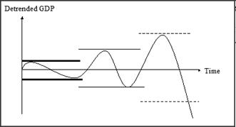
Fig. 6. De-trended GDP – symmetric fluctuations
Fig. 6 shows the case where economy undergoes basic cycles of symmetrically widening amplitude prior to the crisis. However, there is no requirement for this. Another possibility is that cycles have asymmetrically changing amplitude. This alternative case is shown in Fig. 7 which represents Minsky's endogenous financial instability hypothesis as having an upward bias. In this case thwarting institution ceilings are less durable than the floors, giving rise to stronger and longer booms before crisis eventually hits. A third possibility is a long-cycle of constant amplitude and symmetric gradual weakening of thwarting institutions that eventually ends with a financial crisis. This richness of dynamic possibilities speaks to both the theoretical generality and historical specificity of Minsky's analytical perspective. The dynamics of the process are general but how the process actually plays out is historically and institutionally specific.
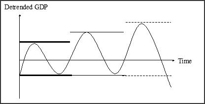
Fig. 7. De-trended GDP – asymmetric fluctuations
Analytically, the full Minsky system can be thought of as a combination of three different approaches to the business cycle. The dynamic behind the Minsky basic cycle is a finance-driven version of Samuelson's (1939) multiplier-accelerator formulation of the business cycle (see Section 3.4). This dynamic is essentially the same as that contained in new Keynesian financial accelerator business cycle models (Bernanke et al. 1996, 1999; Kiyotaki and Moore 1997). Thwarting institution floors and ceilings link Minsky's thinking to Hicks' (1950) construction of the trade cycle. The thwarting institutions are explicitly present in the floors and ceilings, but they can also be present in the coefficients of the multiplier-accelerator model, which determine the responsiveness of economic activity to changes in such variables as expectations and asset prices. Shifting and weakening of floors and ceilings and changing of the behavioral coefficients then capture the long-cycle aspect. This connects Minsky to long wave theory, with the role of financial innovation linking to Schumpeter's (1939) construction of an innovation cycle.
Despite these commonalities with the existing cycle theory, formally modeling Minsky's financial instability hypothesis is difficult and can be potentially misleading. Though models can add to understanding, they can also mislead and subtract.
One problem is that formal modeling imposes too deterministic phase length on what is in reality a historically idiosyncratic process. Adding stochastic disturbances jostles the process but does not adequately capture its idiosyncratic character, which Heraclitus described as ‘No man ever steps in the same river twice’. A second modeling problem is that the timing of real world financial disruptions can appear almost accidental. This makes it seem as if the crisis is accidental when it is, in fact, rooted systematically in prior structural developments, which had generated vulnerabilities.
A third problem is the financial instability hypothesis is a quintessentially non-equilibrium phenomenon in which the economic process is characterized by the gradual inevitable evolution of instability that agents are blind too, even though it is inherent in the structure and patterns of behavior – and agents may even know this intellectually.
This problematic of non-equilibrium is explicitly raised by Minsky (1992b: 104) in his ‘Schumpeter and Finance’ essay, ‘No doctrine, no vision that reduces economics to the study of equilibrium seeking and sustaining systems can have long-lasting relevance. The message of Schumpeter is that history does not lead to an end of history’.
5. Empirical Evaluation of the Cycle Theories of Different Time Scales
Next we discuss some methodology used in the extraction of cycles from data. In the literature there are three typical methods to empirically study cycles. These are, first, spectral analysis (Fourier's theorem), second, filtering methods (HP – filter, BP – filter and penalized splines), and, third, wavelet theory.[9] Since the advantages and disadvantages of the second one have been discussed widely, we will here more extensively focus on the first and the third methods.
5.1. A general approach of extracting cycles from data: Fourier's theorem
Generally speaking, a function is termed periodic if it exhibits the following properties:
f(х) = f(x + T).
In this case, T is known as the ‘period’ and, if x is time, then is the frequency. In the physical world there are many phenomena that exhibit periodic behavior, for example, pendulums, springs, and waves, to name just a few. Mathematical examples also abound.
It is interesting to consider what happens when periodic functions are added together. When several periodic functions are added together, some parts reinforce each other (when both are positive) and other parts cancel each other (when the functions are of opposite sign). But the interactions may be more or less complex and form surprising shapes, for example, a square wave.
From the physical world, we can readily observe certain properties of periodic phenomenon, for example, cancellation, reinforcement, damping, etc. When one moves away from two sound sources emitting tones of different frequencies, one hears, alternately, louder and softer tones.
It was observations of this kind that motivated Joseph Fourier, in the early 1800s to speculate that virtually any function could be formed by adding together the correct combination of periodic functions. In his famous analysis, Fourier defined a sequence of trigonometric values as follows: for any function, f, which is integrable from –π to π
All things come in seasons – Heraclitus
One can never step into the same river twice – Heraclitus
1. Introduction
After a thirty year period of relative tranquility in the world economy – the so-called period of ‘great moderation’ – the U.S. economy suffered a financial meltdown in 2008 that triggered the ‘great recession’. These events have motivated new interest in theories that can explain long periods of expansion that end suddenly with deep recessions. One approach, which has been intellectually unfashionable for many years, is the theory of long economic waves.
This paper examines the empirical and epistemological contributions made by economists regarding the cyclical nature of economic and social development. The paper discusses the main mechanisms of economic cycles involving different time scales, with a particular focus on long wave theory. As part of this survey, the paper shows the continuing relevance of the theoretical constructs developed by Nikolai Kondratieff (also, Kondratiev, Кондратьев) and Simon Kuznets (Кузнец), both for modern macroeconomics and for assessing possible future scenarios. The paper also shows the difficulty of modeling long wave analysis as it poses significant challenges to the equilibrium method which dominates shorter period economic analysis.
Empirical economists and economic historians have voiced diverse views on economic cycles. On the one hand, there seems to be good evidence for business cycles based on a shorter time scale, and the endogenous dynamics of shorter cycles appear to be clear and distinct. On the other hand, long wave cycles are more controversial, involve different theoretical mechanisms, and are harder to verify empirically – in part because data is inevitably more limited owing to the reduced frequency of such cycles. Several different theories of the long wave exist. These include Kondratieff's theory of cycles in production and relative prices; Kuznets' theory of cycles arising from infrastructure investments; Schumpeter's theory of cycles due to waves of technological innovation; Keynes–Kaldor–Kalecki demand and investment oriented theories of cycles; Goodwin's theory of cyclical growth based on employment and wage share dynamics; and Minsky's financial instability hypothesis whereby capitalist economies show a genetic propensity to boom-bust cycles.
Business cycles of shorter duration can be explained by inherent mechanisms that generate cyclical fluctuations in economic activity. However, the mechanical view of long waves is more problematic and challenging. We discuss both those challenges and a recently ‘discovered’ evidence regarding components of long duration cycles. The notion of a financially based long wave Minsky super-cycle, which has been largely overlooked by contemporary economist, appears to have become more relevant in the wake of the financial crisis and the end of the ‘Great Moderation’.
The paper is organized as follows. Section 2 examines the long wave theories of Kondratieff and Kuznets. Section 3 builds on the preceding discussion and analyzes varying time scales and mechanisms of economic cycles prevalent in economic theory. Section 4 examines a Minsky-type of long-period cycles. Section 5 discusses the methodological and empirical challenges involved in detecting economic cycles, particularly those of long duration. Section 6 concludes the paper.
2. The Legacy of Kondratieff and Kuznets
2.1. Kondratieff and theory of long waves
Writing in the early 1920s Nikolai Kondratieff advanced the idea of the probable existence of long wave cycles in capitalist economies lasting roughly between 48 and 60 years. Within that, there is a period of accumulation of material wealth as productive forces move to a newer, higher, level of development. But at a certain point there commences a decline in economic activity, only to re-start growing again later (Kondratieff 2004 [1922]). This mechanism has been dubbed, in economic literature, as Kondratieff cycles.
It should be noted that prior to Kondratieff, some empirical efforts on systematizing the cyclicality of economic crises was carried out by van Gelderen (1913), Buniatian (1915), and de Wolff (1924), which Kondratieff admits to in his publications (see end note in Kondratieff 1935). Though Kondratieff's ideas were not well accepted by the official Soviet economics he insisted on his main argument and in short time followed up with more rigorous publications. Only few English language translations were available at the time (most notably, Kondratieff 1935). Nevertheless, the potency of his ideas was recognized quickly entering the work of subsequent economists (e.g., Schumpeter 2007 [1934]; Kuznets 1971; Rostow 1975; and others) as we review in the next section.
The gist of Kondratieff's argument came from his empirical analysis of the macroeconomic performance of the USA, England, France, and Germany between 1790 and 1920. The economist looked at the wholesale price levels, interest rate, production and consumption of coal and pig iron, production of lead for each economy and price movements (Kondratieff 1935). Using a peculiar statistical method – de-trending the data first and then using an averaging technique of nine years to eliminate the trend as well as shorter waves of Kitchin (Kitchin 1923) type – Kondratieff suggested a regularity of ups and downs in the data on a long time scale. Within that there were intermediate waves along with long waves. As a result, Kondratieff stated that economic process was a process of continuous development. Among possible explanations to the long wave cycles Kondratieff mentions: a) changes in technology; b) wars and revolutions; c) appearance of new countries on the world map; and d) fluctuations in production of gold (Kondratieff 1935, 2002).
All four appear as valid external shocks in pushing any particular economy or the world economy into a downward or upward cycle path. However, after careful analysis it became evident that external factors could not be the sole determinants of shocks in economic transformation. The missing part is the accumulation of preceding events, and the development of economic – but also social, and political – relationships over long cycles that may help to endogenize the external factors.
Fig. 1a illustrates an approximation of Kondratieff's original timeline of long wave cycles. Kondratieff's original estimation was based on a commodity prices index for the USA, England, and France in his work of 1935 (see Kondratieff 1935). Subsequently, with popularization of Kondratieff's views, extensions to the original analysis, roughly following the 40–60 years rule, began to appear.
Fig. 1a. Long waves cycles illustration
Source: authors' approximation based on Kondratieff (1935).
One of the first to catch on the logic was Schumpeter (1939) who pointed out the distinction between short (Kitchin cycles of 3–4 years), medium (Juglar cycles of 9–10 years),[1] and long (Kondratieff cycles of 54–60 years) cycles in his analysis of economic development. We discuss some of them below.
As to mechanisms, Kondratieff already pointed to a large-scale accumulation of innovative activity, that is inventions and processes modifications that required fifty or more years before complete insertion, absorption in the production method. The role of innovation, implied in Kondratieff's analysis, is captured by the internal dynamic tendencies described in detail in Schumpeter's The Theory of Economic Development (Schumpeter 2007 [1934]). In turn, Garvy (1943) subjects Kondratieff's proposition to sharp criticism from positions of Soviet economists and from the point of view of Western economics. Paradoxically, in either case the conclusion appears to be that Kondratieff was too hasty in assigning the term ‘cycle’ to his propositions, as those do not correspond to the internal evolutionary dynamics following some mechanism of cycles.
There was a difference however in the Western economists' views and their contemporary Soviet counterparts. From the Western economist point of view, articulated by Garvy (Ibid.), there was no sufficient statistical evidence to warrant any regularity, that is cyclicality, to Kondratieff's analysis. The Soviet economists writing around the time of Kondratieff's original publications and shortly after (e.g., Studensky, Oparin, Pervushin, Bogdanov, Sukhanov and others, see Garvy 1943 for concise discussion and references) rejected the term ‘cycle’ in reference to the capitalist production mode since that implied some type of capitalist system's perpetuity. At the time that was in direct opposition with the socialist beliefs of gradual phasing out of the capitalist economy into its next logical stage of socialism, as was implied by then dominant interpretation of Marx's Capital (2003 [1867]). These beliefs in rapid phased successions picked up from simplistic interpretations would feed into initial enthusiasm around shock therapy reforms in post-socialist economies in the early 1990s (Gevorkyan 2011).
Recently, researchers working within Kondratieff's original methodological scope have attempted to extend their analysis across the twentieth century with focus on predictive capabilities of such work into the nearest future. Some find the ongoing economic deterioration in the world economy fitting calculations of the Fifth Long Wave of the Kondratieff cycle (e.g., Korotayev and Tsirel 2010; Kondratieff 2002; Akaev 2009; and others), some of them using spectral analysis. A re-validation of the very four exogenous shocks (technology, wars, shifts in boundaries, and value of gold) so carefully documented and refuted by Kondratieff himself took place in some of those papers. Exogenous shocks are surely important ‘occurrences’, yet, the internal dynamics in the evolution of economic relationships over a long time period and staging economic development must be considered as well. We address this in further detail below, using more modern empirical methods.
2.2. Kuznets' novel analysis of development
Simon Kuznets received the Nobel Prize in Economics in 1971 for his empirical analysis of economic growth, where he identified a new era of ‘modern economic growth’. Like Kondratieff, Kuznets relied on empirical analysis and statistical data in his pioneering research. Absorbing his findings on historical development of the industrial nations with initially abstract categories of the national income decomposition, Kuznets developed a concept of long swings, though disputed, now referred to as Kuznets cycles or Kuznets swings (e.g., Korotayev and Tsirel 2010).
The Kuznets swings' period is ranged between 15–25 years and initially connected by Kuznets with demographic cycles. In that analysis, the economist observed and quantified the cyclicality of production and prices, linking with immigrant population flows and construction cycles. Researchers have attempted to connect these cycles with investments in fixed capital or infrastructure investments (see Ibid. for literature review). Focusing on developed economies of North America and Western Europe, Kuznets computed national income from late 1860 forward with structural breakdowns by industry and final products. He also provided measures of income distribution between rich and poor population groups.
Kuznets unveiled the deficiency of constrained theoretical work built on simplified assumptions. He was critical of capital and labor as the sole factors sufficient for economic growth. Instead analysis must encompass information on technology, population and labor force skills, trade, markets, and government structure. Kuznets carried his analysis further in developing measures of national income through categories of consumption, savings, and investment (e.g., Kuznets 1949, 1937, 1934, etc.), eventually leading to a system of national income accounting.
It should also be noted that while working on the problem of income inequality, Kuznets was one of the first to look at economic growth measurements in the developing world (e.g., Kuznets 1971, 1966, and 1955). His well-known inverted U-shaped curve measuring inequality on the y-axis and economic development, expressed as change in GNP on the x-axis was an intellectual breakthrough of the time (see Fig. 1b). The conclusion is that while the economy remains in agricultural stage income inequality among different groups within the economy is low. As the national economy embarks on the process of industrialization inequality rises over time, then it falls again.
Fig. 1b. Kuznets curve
This describes the experience of developed economies in Western Europe and North America, that is the initial phases of industrialization cause sharp rises in inequality. Upon reaching a critical saturation point, inequality subsides while economic growth continues. This happens through the emergence of a ‘middle class’, improved education facilities, health care, and governance. It is interesting to note that further structural change and the shifting of resources to services and the financial sector, may increase inequality again, as, for example, is seen in the U.S. economy since the 1980s. It may be argued that this somewhat correlates to a popular analysis in development economics on the transition mechanisms from traditional to modern industrial sectors.
A variant of the Kuznets curve is also utilized in the analysis of environmental problems. This application suggests an immediate deterioration in air quality and intensification of environmental problems at the initial industrializing stages until spreading affluence and emergence of middle class introduces legislative and other controls on hazardous production (WB 1992; Grossman and Krueger 1995 and more recently Stern 2004). Elsewhere, these implied predictions of fading inequality offered a strong intellectual foundation for the mentioned reforms of the early 1990s in Eastern Europe and the former Soviet Union (Gevorkyan 2011). In studies of sequencing of market liberalization reforms and limitations of the state in the economy there were omitted the negative externalities of shock therapy policies. Yet, in the early 1990s, the promise of immediate market reforms and potential access to greater income opportunities did not materialize at the height of the reforms. In fact, income inequality problems still remain relevant and critical on policymakers' agendas two decades since the ‘transition’. The absence of the universal tendency of declining income inequality raises a question of how one measures economic development and what time-frame to consider is ‘sufficient’ to measure the rise of ‘welfare’ over time.
Finally, Kuznets (1973) brings up six key characteristics of modern economic growth, based on methodology consistent with national income accounting and historical analysis of economic development: 1) increase in per capita growth and population in developed economies; 2) increasing productivity rates; 3) increasing rate of structural transformation; 4) rising urbanization and secularization; 5) spread of technology and infrastructure improvements (communications); 6) limits to wide-scale spread of economic growth and benefits. Therefore despite seeming improvements, Kuznets noted persistence of disproportionate economic growth worldwide and apparently some broader measures of welfare.
Broadly speaking, such persistence of long wave-like tendencies on a global scale, a feature of contemporary industrial and financial globalization, supports the concept of redefined fundamental uncertainty (Gevorkyan and Gevorkyan 2012). Here the uncertainty of the direction, length, and capability of the post-great recession's potential recovery remains unclear. The lesser-developed economies (aka emerging markets) are worst affected in such circumstances, as the speculative foreign capital exits and industrial capacity remains inadequate on global competitive scale with absent technological advance.
Common between the work of both Kondratieff and Kuznets was the motivation to define the mechanisms of economic growth and development, and systematize core tendencies driving the transformational momentum. That in turn connects directly to the earlier discussion on cyclicality in development.
3. Time Scales and Mechanisms of Economic Cycles
As mentioned, the work of Kondratieff and Kuznets fostered a systematic approach to modern understanding of long economic swings. Numerous authors have further proposed not only different mechanisms underlying cycles but also cycles on different time scales. An early theory of cycles was put forward by Robert Owen in 1817, who stressed wealth inequality and poverty, originating in industrialization, yielding under-consumption as a reason for economic crises. Sismondi, in the middle of the 19th century took a similar view and developed a theory of periodic crises due to under-consumption. This led to the discussion of the ‘general glut’ theory of the 19th century, which Marx and other classical economists also extensively contributed to.
More specifically, a mechanism of cycles on a shorter times scale, of 8–10 years duration, was developed by Juglar (Juglar cycles), resulting, as he saw it, from the waves in fixed investment. Later, Kitchin, in the 1920s, introduced an inventory cycle of 3–5 years. Later an important contribution was made by Schumpeter (1939), who referred to the ‘bunching’ of innovations and their diffusion as a cause for long waves in economic activity.
Roughly at the same time, Samuelson (1939), influenced by the Spiethof accelerator and the Keynesian multiplier principle, developed the first mathematically-oriented cycle theory using difference equations.[2] Others, such as Rostow (1975), had proposed the theory of stages of growth. Simultaneous with Samuelson, Kalecki (1937) developed his theory of investment implementation cycles where he saw significant delays between investment decisions and investment implementations, formally introducing differential delay systems as tool for studying cycles.
Kaldor (1940), rooted in Keynesian theory, developed his famous nonlinear investment-saving cycles, which took into account aggregate demand. Later, Goodwin (1967) proposed a model of growth cycles, which took into account classical growth theory, but was based on unemployment-wage share dynamics, since the overall growth rate, as well as productivity growth, are kept constant in the long run. We will first discuss cycle theories on a longer time scale and then move to the Goodwin and Keynes-Kaldor cycles. We also briefly include a discussion of Kalecki's cycle theory (1971) and how it might relate to Kondratieff.
3.1. The Kondratieff long swings
The above review raises a few critical questions that need proper evaluation. For example, it is difficult to detect clear mechanisms in the Kondratieff cycles (e.g., as sketched in Fig. 1a above). If anything is working here as a mechanism, it must be some exhaustion of endogenous and exogenous factors: in the long upswing prices are rising, interest rates rise and wages rise, raw materials and non-renewable resources may be exhausted, causing to drive up prices and wages. New technologies are discovered in periods of long down swings, which come to be used in a new upswing. New resources are discovered, such as iron ore, coal, gold and other metals, which Kondratieff argues to be endogenously expanded through new discoveries but both technology and resources will finally be exhausted too: resource and product prices rise, deposits at saving banks rise, but also interest rates and wages rise and a downturn begins. There is a struggle for markets and resources. New countries are opened up. There are market limits, such export limits, which restrict further expansions, as Kondratieff data on French exports show. Then, in the long downswing, prices fall, wages fall, interest rates fall, plenty of resources and unused production capacity push prices down, and unemployment reduces wages. Overall, there are some mechanisms indicated in Kondratieff, but not specifically modeled.
3.2. The Kuznets long swings
Further, Kuznets theory of development and fluctuations can be seen as an interesting intersection of two traditions in the economics of his time. On the one hand, he was interested in cyclical movements in numerous time series data, such as volume of all types of production and prices, seasonal and secular movements in industry income and national income and its components, long swings in economic activities, and business cycle analysis. On the other hand, he saw development as a time irreversible process of industry and national income development, which evolves in stages of economic growth, with plenty of structural changes. Each stage may have its particular saving rate, consumption patterns, unevenness and disequilibrium as well as income inequality. As described above, inequality first rises with industrialization and later declines. Kuznets conceptual framework can be seen as a mixture of cycle theories, referring to the accelerator principle for infrastructure investments, and a theory of stages of economic growth that were similar to those pursued by Rostow (1975). A similar view on stages of growth, that taken by Kuznets and Rostow, is also pursued by Greiner, Semmler and Gong (2005). Overall, Kuznets was ambiguous whether there are regular mechanisms generating cycles. He conjectured that cycles may be in the economic data solely as a result of certain historical ‘occurrences’.
3.3. The Schumpeter innovation cycles
Schumpeter's concept of competition deviates from the neoclassical conception in some essential aspects. First, competition is not limited to price or quantity adjustments. It is described as an evolutionary process, as a process of ‘creative destruction’. The engines of this development are capitalist enterprises. ‘Capitalism, then, is by nature a form or method of economic change and not only never is but never can be stationary ... The fundamental impulse that sets and keeps the capitalist engine in motion comes from the new consumer's goods, the new methods of production or transportation, the new markets, the new forms of industrial organization that capitalist enterprise creates’ (Schumpeter 1970: 83). The incentives for developing these types of technical change originate in transient surplus profits. What is taken as given in neoclassical general equilibrium analysis as parametric data, when the price and quantity adjustments occur is the explicandum in Schumpeter: process innovation, product innovation, new forms of organization of the firm and new forms of financial control.
Second, Schumpeter stresses that competition is not necessarily an equilibrating force. When referring to the existence of entrepreneurial firms and their rivalry, Schumpeter maintains that ‘there is in fact no determinate equilibrium at all and the possibility presents itself that there may be an endless sequence of moves and counter-moves, an indefinite state of warfare between firms’ (Ibid.: 79). Moreover, competition as an evolutionary process takes place through time, in discrete steps. For example, he writes, ‘Now the first thing we discover in working out the propositions that thus relate quantities belonging to different points in time is the fact that, once equilibrium has been destroyed by some disturbances, the process of establishing a new one is not so sure and prompt and economical as the old theory of perfect competition made it out to be, and the possibility that the very struggle for adjustment might lead such system farther away instead of nearer to a new equilibrium. This will happen in most cases unless the disturbance is small’ (Ibid.: 103). Indeed, in Schumpeter it is the product and process innovation, undertaken by the entrepreneur, which brings the economic system out of equilibrium, resulting in long waves and business cycles. Moreover, he even does not seem to be very interested in a theory of centers of gravitation for market forces as developed by the classical economists.
Third, in Schumpeter, competition is an evolutionary process, one of rivalry between firms motivated by the search for surplus profit. He calls this surplus profit the transient ‘monopoly profit’ of new processes and new products, ‘Thus, it is true that there is or may be an element of genuine monopoly gain in those entrepreneurial profits which are the prizes offered by capitalist society to the successful innovator. But the quantitative importance of that element, its volatile nature and its function in the process in which it emerges put it in a class by itself’ (Ibid.: 102). ‘The transient surplus profit does not appear as deviation from the perfectly competitive state of the economy and as a waste in the allocation of resources, but as a reward for the innovator and a gain for the capitalist society. On the contrary, the perfectly competitive economy, where every market agent behaves in the same way under the condition of parametrically given external conditions seems to imply a waste of resources ... working in the conditions of capitalist evolution, the perfect competitive arrangement displays wastes of its own. The firm of the type that is compatible with perfect competition is in many cases inferior in internal, especially technological, efficiency. If it is, then it wastes opportunities’ (Schumpeter 1970: 106). Thus, in Schumpeter's view, the entrepreneurial firms are powerful engines of progress and ‘in particular of the long-run expansion of total output’ (Ibid.).
Following Schumpeter's footsteps, the literature after Schumpeter has distinguished between radical and incremental innovation. The major waves of radical innovations, which were followed by the diffusion of this new technology and incremental innovations are.[3]
· The water-powered mechanization of the industry of the 18th and early 19th century;
· The steam-powered mechanization of the industry and transport of the middle of the 19th century (rail ways, steam engines, machine tools);
· The electrification of industry, transport and homes at the end of the 19th century;
· Motorization of industrial production, transport, civil economy and the war machinery (from ~1914 onward);
· Computerization and information technology from the 1960s and 1970s onward.
According to Schumpeter's oriented long wave theories, each of those radical innovations did not only create long waves in economic development, but each of those long waves were driven by different technology, originated in different countries and then diffused world wide.
3.4. The Samuelson accelerator-multiplier cycles
A model of medium-time scale is the one created by Samuelson (1939). The basic construction is as follows: consumer spending (via increased sales by firms) accelerates investment; output changes results in income changes through the multiplier, which, in turn, again stimulates sales, that is consumer spending.
The multiplier-accelerator model of Samuelson (Ibid.) can produce cycles. Take Сt = consumption, It = investment, Yt = income, C0 = autonomous consumption, I0 = autonomous investment, and G = C0 + I0; I = S = sY, therefore the multiplier is: ![]() Use:
Use:
Ct = C0 + ?Yt – 1, (1)
It = I0 + ? (Yt – 1 – Yt – 1), (2)
Yt = Сt + It . (3)
Substituting (1) and (2) into (3) gives
Yt = С0 + ?Yt – 1 + I0 + ?Yt – 1 – ?Yt – 2,
G = C0 + I0,
Yt = G + (? + ?) Yt – 1 – ?Yt – 2.
The standard form of a second order linear difference equation is:
Yt – (? – ?) Yt – 1 + ?Yt – 2 = G, (4)
which is stable or unstable depending on the size of ?. Moreover, one can have contracting or expanding cycles depending on whether there exist imaginary parts of the eigenvalues (see Figs 2a – 2d).
When we replace income by profit flows Rt, one can turn the above into a kind of Kalecki model such as: It + 1 = A + ?Rt + b(Rt – Rt – 1). If one writes for spRt = It, ![]() , we get a similar second order difference equation:
, we get a similar second order difference equation:
![]() , (5)
, (5)
which again can be stable or unstable and it can produce unidirectional change or oscillations. The Kalecki model is further studied in Sub-section 3.7.
Figs 2a – 2d. Stable and unstable development and oscillations
3.5. The Goodwin growth and income distribution cycles
Other types of cycles that have been discussed, particularly in the Post War II period, where Goodwin's growth cycle theory that postulates an interaction of employment and wage share. It looked like a business cycle model when it was first proposed but, in fact, empirically it seems to operate also on a medium time scale.[4]
Goodwin (1967) postulates cycles driven by growth and income distribution. Low growth, generated by low profits and investment, generates unemployment, which in turn limits wage growth as compared to productivity. This gives rise to lowering the wage share: low wage share means high profit share and slowly rising investment, which reaches a turning point as employment and wage growth make the wage share rising and the profit share falling. By utilizing nonlinear differential equations, originally developed by Lotka and Volterra for the models of interacting populations, we can rewrite the Goodwin model of wage-employment dynamics as follows:
![]() ,
,
or as
,
where ![]() represents the time rate of change of the ratio of the employed to the total labor force and
represents the time rate of change of the ratio of the employed to the total labor force and ![]() is the change of the wage share. Both variables depend on the level of х and the constants a, b, c, d > 0. The coefficient, a, denotes the trend of employment if all income is reinvested (y = 0) and d is the fall in real wage if (x = 0). The symbol by denotes the influence of the wage share on the employment ratio, and cx the positive influence of employment on the wage share. Due to this interaction of the variables the employment ratio is prevented from rising and the wage share from falling without limits.
is the change of the wage share. Both variables depend on the level of х and the constants a, b, c, d > 0. The coefficient, a, denotes the trend of employment if all income is reinvested (y = 0) and d is the fall in real wage if (x = 0). The symbol by denotes the influence of the wage share on the employment ratio, and cx the positive influence of employment on the wage share. Due to this interaction of the variables the employment ratio is prevented from rising and the wage share from falling without limits.
For a growth model with trends as represented by Goodwin, the coefficients can be interpreted as follows: a = b – (m + n) where b is the output/capital ratio (Y/K), m is the growth rate of productivity and n is the growth rate of the labor force. All of those are taken as constants. Assuming a linearized wage function (for instance, ![]() and with m the growth rate of productivity as before, we obtain for the growth rate of the wage share the term
and with m the growth rate of productivity as before, we obtain for the growth rate of the wage share the term ![]() with m = d – e. Thus, the second pair of differential equations can be written as:
with m = d – e. Thus, the second pair of differential equations can be written as:
![]()
![]()
which is indeed equivalent to the first equation of the (above) system, except that it is written in terms of growth rates. The core of the last system shows that the change of the employment ratio depends on the profit share (1 – y) and that the change of the wage share depends on the employment ratio. This form has been used to explain the fluctuation of the employment ratio and the fluctuation of the industrial reserve army in Marx (Marx 2003 [1867]: ch. 23; see Goodwin 1967). The basic structure of this model represents the interacting variables of the employment ratio and wage share as dynamically connected.
The last system has two equilibria: (0, 0) and ![]() . The linear approximation of the system is with ?1, ?2 as small deviations from the equilibrium values
. The linear approximation of the system is with ?1, ?2 as small deviations from the equilibrium values
![]() .
.
The calculation of the Jacobian for the first linear approximation gives for the equilibrium ![]()
The real parts of the eigenvalues are zero and the linear approximation of the equilibrium point represents the dynamical structure of a center (Hirsch and Smale 1974: 258). With real parts of the eigenvalues zero, the linear approximation of the system through the Jacobian does not allow conclusions regarding the behavior of the dynamical system in the neighborhood of the equilibrium. Yet, as can be shown, by constructing a Liapunov function for the above system, which is constant in motion and hence has time derivatives ![]() the wage share-employment dynamics results in closed solution curves (Ibid.; Flaschel and Semmler 1987).
the wage share-employment dynamics results in closed solution curves (Ibid.; Flaschel and Semmler 1987).
The closed trajectories of the system are, however, only closed curves and the wage share-employment dynamics does not allow for persistent cycles, such as limit cycles (Hirsch and Smale 1974: 262; Flaschel 1984). In addition (see Flaschel and Semmler 1987), the dynamical system is structurally unstable, since small perturbations can lead to additional interaction of the variables (J11 or J22 can become nonzero). This leads to a qualitatively different dynamical behavior of the system, hence it can become totally stable or unstable. Under certain conditions the above system can also become globally asymptotically stable. This can occur if the conditions for Olech's theorem are fulfilled (see Flaschel 1984).
Equivalent results are obtained when in place of a linear wage function a nonlinear wage function is substituted in the system (see Velupillai 1979). The wage share-employment dynamics worked out originally by Goodwin for a model of cyclical growth and then applied by him to explain an endogenously created unemployment of labor depict a growing economy, whereas often models of nonlinear oscillations refer only to a stationary economy.
Since the change of the wage share and the change of labor market institutions such as bargaining and other protective legislature are slow, this model of economic cycles, however, does not really model business cycles but rather medium run cycles. On the other hand, for a theory of longer cycles the dynamical interaction of other important variables over time (such as waves of innovations, changes of capital/output ratio, productivity, relative prices and interest rates) as well as demand factors are neglected.
3.6. The Keynes–Kaldor demand driven cycles
The demand factors are considered in the next section presented here. The Keynes–Kaldor model seems to operate on a shorter time scale. It essentially refers to the role of demand, defined by the relation of investment and savings. In his article, Kaldor (1940) proposed such a shorter scale cycle model, a nonlinear model of business cycles, which after that has been reformulated in the light of mathematical advances in the theory of nonlinear oscillations, which take into account demand changes (Kaldor 1940, 1971; Chang and Smyth 1971; Semmler 1986).
Kaldor relies on a geometric presentation of a business cycle model which depends on a nonlinear relation between income changes and capital stock changes and which seems to generate self-sustained cycles without rigid specifications for the coefficients, time lags and initial shocks. The geometric presentation of his model of persistent business cycles due to the dynamic interaction between income changes and accumulation and dissolution of capital indeed also includes the possibility of limit cycles, that is asymptotically stable cycles regardless of the initial shocks and time lags.
His ideas are also formulated for a stationary economic system and can be represented by nonlinear differential equations in the following way (Chang and Smyth 1971):
![]()
where ? is a reaction coefficient, ![]() the rate of change of income,
the rate of change of income, ![]() the rate of change of the capital stock, I = investment and S = saving as functions of the level of income and capital stock. According to the assumptions underlying the model, there is a unique singular point (Ibid.: 40). This type of Keynesian–Kaldorian model can give rise to persistent cycles (see Semmler 1986), it does not model the specific role of growth and income distribution, as Goodwin has stressed. Yet it stresses the role of endogenously changing demand. The linear approximation is:
the rate of change of the capital stock, I = investment and S = saving as functions of the level of income and capital stock. According to the assumptions underlying the model, there is a unique singular point (Ibid.: 40). This type of Keynesian–Kaldorian model can give rise to persistent cycles (see Semmler 1986), it does not model the specific role of growth and income distribution, as Goodwin has stressed. Yet it stresses the role of endogenously changing demand. The linear approximation is:
![]() ,
,
where the Jacobian is
,
where ![]() since
since ![]() and
and ![]() (Chang and Smyth 1971: 41). The determinant is
(Chang and Smyth 1971: 41). The determinant is ![]() which is positive because for the existence of a unique singular point it is assumed that
which is positive because for the existence of a unique singular point it is assumed that ![]() . The element,
. The element,![]() , is always negative. The linear approximation with the Jacobian represents at its core the investment-income dynamics according to which the change of income depends negatively on the level of the capital stock
, is always negative. The linear approximation with the Jacobian represents at its core the investment-income dynamics according to which the change of income depends negatively on the level of the capital stock ![]() and the change of capital stock depends positively on the level of income
and the change of capital stock depends positively on the level of income ![]() but there is a negative feedback effect from the level of capital stock to the change of capital stock and an ambiguous feedback effect from the level of income to the change of income
but there is a negative feedback effect from the level of capital stock to the change of capital stock and an ambiguous feedback effect from the level of income to the change of income ![]() . This will be explained subsequently.
. This will be explained subsequently.
Analyzing the singular point one can conclude that the equilibrium is a focus or a node and that the equilibrium is stable or unstable accordingly as ![]() This singular point also allows for a limit cycle, since the necessary condition for a limit cycle is that the dynamic system has an index of a closed orbit, equal to 1 (Minorsky 1962: 79). This excludes a saddle point as a singular point (see Ibid.: 77). Moreover, the most interesting point in this dynamic system is the ambiguous element
This singular point also allows for a limit cycle, since the necessary condition for a limit cycle is that the dynamic system has an index of a closed orbit, equal to 1 (Minorsky 1962: 79). This excludes a saddle point as a singular point (see Ibid.: 77). Moreover, the most interesting point in this dynamic system is the ambiguous element ![]() . According to Kaldor's graphical presentation, it is assumed (see Kaldor 1940: 184) that
. According to Kaldor's graphical presentation, it is assumed (see Kaldor 1940: 184) that
(1) ![]() for a normal level of income;
for a normal level of income;
(2) ![]() for abnormally high or abnormal lowly levels of income; and
for abnormally high or abnormal lowly levels of income; and
(3) the stationary state equilibrium has a normal level of income.
Fig. 3. Kaldor graph on nonlinear investment and saving functions
This might be illustrated by Fig. 3 with Y being the level of output, which shows that the normal level of Y is unstable and the extreme values of Y are stable. Mathematically this means that the trace ![]() changes signs during cycles. This is the negative criterion of Bendixson (Minorsky 1962: 82) for limit cycles, that is if the trace
changes signs during cycles. This is the negative criterion of Bendixson (Minorsky 1962: 82) for limit cycles, that is if the trace ![]() does not change signs, persistent cycles – limit cycles – cannot exist (see also Guckenheimer and Holms 1983: 44). As proven by Chang and Smyth (1971: section V), there indeed exists the possibility of stable cycles, limit cycles, under the assumption proposed by Kaldor.
does not change signs, persistent cycles – limit cycles – cannot exist (see also Guckenheimer and Holms 1983: 44). As proven by Chang and Smyth (1971: section V), there indeed exists the possibility of stable cycles, limit cycles, under the assumption proposed by Kaldor.
However, the three conditions as formulated above and originally formulated by Kaldor (1940: 1984) are not necessary for the existence of cycles. What is actually necessary for cycles is only that ![]() (i.e. that
(i.e. that ![]() switches signs) at some level of Y. Moreover, the singular point at the normal level of Y does not have to be unstable as a necessary condition for a limit cycle. The critical point can be stable (see Minorsky 1962: 75). In addition there also is the possibility that the system is globally asymptotically stable. This is the case if:
switches signs) at some level of Y. Moreover, the singular point at the normal level of Y does not have to be unstable as a necessary condition for a limit cycle. The critical point can be stable (see Minorsky 1962: 75). In addition there also is the possibility that the system is globally asymptotically stable. This is the case if: ![]() and (2)
and (2) ![]() everywhere.
everywhere.
The global asymptotic stability under these conditions follows from Olech's theorem (see Ito 1978: 312).
Evaluating Keynes–Kaldor's model of a demand driven business cycles one can say that Kaldor's formulation of an income-investment dynamics brought some advances regarding a theory of endogenously produced business cycles, especially formulations of the theory of cycles in terms of a theory of nonlinear oscillations (see also Kaldor 1971) one can extend this to include a formulation concerning the dynamics in employment and wage share which was originally more visible in classical models that referred to the profit-investment dynamics.
3.7. The Kalecki profit and investment cycles
To draw some similarities to the Kondratieff long wave theory, we can follow Kalecki (1971) and replace the income, Y, by profit flows П[5] and allow for ![]() to change its sign during the cycle. In some sense the role of profit, wages and income distribution – as in the Goodwin model – can be allowed to come in here.
to change its sign during the cycle. In some sense the role of profit, wages and income distribution – as in the Goodwin model – can be allowed to come in here.
In general it could be assumed that:
(Case 1) ![]() for profit income in an interval such as П1 < П < П2 (see Fig. 4). This may be due to a previous decrease in capital stock, production and employment which entail low construction cost for plants, low material and resource cost and low wage costs (relative to productivity), high profits and low interest rates and easy access to credit. These factors then may give rise to an expectation of rising profits on investments.
for profit income in an interval such as П1 < П < П2 (see Fig. 4). This may be due to a previous decrease in capital stock, production and employment which entail low construction cost for plants, low material and resource cost and low wage costs (relative to productivity), high profits and low interest rates and easy access to credit. These factors then may give rise to an expectation of rising profits on investments.
On the other hand, in other regions we can have:
(Case 2) ![]() with two clarifying conditions:
with two clarifying conditions:
(a) for П > П2 due to capacity limits, rising construction cost for plants and rising material and wage cost (relative to productivity), exhaustion of exhaustible resources, rising interest rates and but falling actual and expected profits. Profits and expected profits may fall due to the rise of those costs and wages – that cannot be passed on – in the long upswing. This looks similar to a mechanism that Kondratieff has indicated to eventually occur in his long upswing (see Sections 2.1 and 3.1).
(b) for П < П1 in a recessionary or slow recovery period, where firms invest in financial funds instead of in real capital (Minsky 1983) but due to the economic conditions in a recessionary period, the rate of change of saving in response to falling profits tend to drop faster than the rate of change of investment. Wage share may have been rising previously, and profit share falling but here investment is still not dropping completely to zero. This resembles the Kondratieff scenario of a long downswing and recessionary or stagnation period.
Though the economic intuition appears the same in our above stylized business cycle dynamics and the Kondratieff long waves phases, the time scales are probably different ones: one is a shorter one and the other a longer one, but the mechanisms may be the same. Yet, for a longer time scale much of the economic structure and relationships are likely to change.
In the history of economic thought the change of sign for ![]() during the economic cycle was verbally anticipated by many writers on the study of capitalist dynamics (Kalecki 1971: 123; Kaldor 1940: 184) and can be regarded as essential for a theory of fluctuations in economic development. Mathematically
during the economic cycle was verbally anticipated by many writers on the study of capitalist dynamics (Kalecki 1971: 123; Kaldor 1940: 184) and can be regarded as essential for a theory of fluctuations in economic development. Mathematically ![]() must change signs in order to generate self-sustained cycles. If
must change signs in order to generate self-sustained cycles. If ![]() and
and ![]() were zero,
were zero, ![]() and
and ![]() alone would determine the profit-investment dynamics. There would only be structurally unstable harmonic oscillations. The negative signs of
alone would determine the profit-investment dynamics. There would only be structurally unstable harmonic oscillations. The negative signs of ![]() and
and ![]() exert a retarding influence on accumulation, and
exert a retarding influence on accumulation, and ![]() represents an accelerating force on capital accumulation, whereas
represents an accelerating force on capital accumulation, whereas ![]() exerts a retarding influence in the boom period and an accelerating impact on profit and accumulation in the later phase of the recession.
exerts a retarding influence in the boom period and an accelerating impact on profit and accumulation in the later phase of the recession.
Intuitively, the existence of self-sustained cycles can be seen in Fig. 4 from the fact that the trajectories of П(t) and К(t) are bounded in absolute values and the profit-investment dynamics follow certain directions in the plane. Roughly speaking, for large enough П(t), ![]() turns negative and for large enough К(t),
turns negative and for large enough К(t), ![]() turns negative and vice versa. Geometrically, this is illustrated by Fig. 4.
turns negative and vice versa. Geometrically, this is illustrated by Fig. 4.
Fig. 4. Phase diagram
For ![]() we get the slope
we get the slope
![]() ,
,
and for ![]() the slope is
the slope is
![]() .
.
![]() Thus, in the plane of the Fig. 4 there are four quadrants. For reasons of simplicity we have assumed a linear investment function in Fig. 4. The system has a unique solution at П* and K* since the curve
Thus, in the plane of the Fig. 4 there are four quadrants. For reasons of simplicity we have assumed a linear investment function in Fig. 4. The system has a unique solution at П* and K* since the curve ![]() has a steeper slope than
has a steeper slope than ![]() when the latter is upward sloping in a certain region. This follows from the assumption in the model.[6] The determinant of the Jacobian of the dynamical system above is
when the latter is upward sloping in a certain region. This follows from the assumption in the model.[6] The determinant of the Jacobian of the dynamical system above is ![]() The singular point is a focus or a node and is stable or unstable accordingly as
The singular point is a focus or a node and is stable or unstable accordingly as ![]() < 0. A saddle is excluded, and the singular point has index 1 as necessary condition for a self-sustained cycle (Minorsky 1962: 176). (The singular point does not have to be unstable as Kaldor originally assumed; see Kaldor 1940: 182.) The existence of a self-sustained cycle follows intuitively from the analysis of the vector fields in the different regions, which correspond roughly to stages of economic cycles.[7]
< 0. A saddle is excluded, and the singular point has index 1 as necessary condition for a self-sustained cycle (Minorsky 1962: 176). (The singular point does not have to be unstable as Kaldor originally assumed; see Kaldor 1940: 182.) The existence of a self-sustained cycle follows intuitively from the analysis of the vector fields in the different regions, which correspond roughly to stages of economic cycles.[7]
For region I, which expresses the dynamics of a recovery period, К(t) is below the ![]() curve and П(t) is below the
curve and П(t) is below the ![]() curve; the decline in capital stock and its effect on profit (i.e. the effects of Cases 1 and 2) as well as other changes in economic conditions in a recessionary period will generate a positive rate of change of profit (since
curve; the decline in capital stock and its effect on profit (i.e. the effects of Cases 1 and 2) as well as other changes in economic conditions in a recessionary period will generate a positive rate of change of profit (since ![]() in region I, see also Case 1). Therefore, in region I we will find
in region I, see also Case 1). Therefore, in region I we will find ![]() and
and ![]()
The increase of profits and investments after a recessionary period will lead to rising К(t), but through the effect of Cases 1 and 2 (i.e. the negative effect of growth of capital stock on profits) the growth rate of II will become negative. Thus, in region II, indicating a boom period, we have ![]() and
and ![]() Hence, the arrows in Fig. 4, indicating the direction of the vector field of П and K, will start bending inward (see Case 2a which leads to
Hence, the arrows in Fig. 4, indicating the direction of the vector field of П and K, will start bending inward (see Case 2a which leads to ![]() ). With capital stock rising and
). With capital stock rising and ![]() due to a magnitude of capital stock greater than its stationary value K*, the capital stock must eventually decline (i.e. through the effect of Case 2). We also have
due to a magnitude of capital stock greater than its stationary value K*, the capital stock must eventually decline (i.e. through the effect of Case 2). We also have ![]() due to
due to ![]() at the beginning of a downswing period (capital may be accumulated more as money capital than as real capital).
at the beginning of a downswing period (capital may be accumulated more as money capital than as real capital).
In region III, indicating a downswing period, through the influence of ![]() on K(t), K(t) also starts declining; thus
on K(t), K(t) also starts declining; thus ![]() and
and ![]() Hence, for
Hence, for ![]() and
and ![]() the vector field is pointing inward. A decline of capital stock below K* in region IV, the recessionary period, however, eventually causes profits to rise. The recessionary period may slowly then turn into a recovery period, indicated by region I. This, of course, assumes again that eventually
the vector field is pointing inward. A decline of capital stock below K* in region IV, the recessionary period, however, eventually causes profits to rise. The recessionary period may slowly then turn into a recovery period, indicated by region I. This, of course, assumes again that eventually ![]() . The investment of financial funds turns into investment in real capital, thus investment out of profit tends to become greater than savings out of profit. The recessionary period (with wage increase below productivity, low material and capital cost, low interest rates and easy access to credit as well as a decline in capital stock and thus rising profit expectation[8] must have its impact on
. The investment of financial funds turns into investment in real capital, thus investment out of profit tends to become greater than savings out of profit. The recessionary period (with wage increase below productivity, low material and capital cost, low interest rates and easy access to credit as well as a decline in capital stock and thus rising profit expectation[8] must have its impact on![]() , for otherwise the recessionary period will endure.
, for otherwise the recessionary period will endure.
Therefore, under the economic conditions stated in Cases 1, 2a, and 2b the profit-investment dynamics creates its own cycles by which profit, investment and thus output and employment cannot exceed certain boundaries. The dynamic system is self-correcting and fluctuates within limits: for large enough K(t) is ![]() and for large enough П(t) is
and for large enough П(t) is ![]() . A similar argument holds for small enough K(t) and П(t). Thus, whereas the system with Cases 1 and 2 becomes stable at its outer boundaries (indicated by the negative sign of
. A similar argument holds for small enough K(t) and П(t). Thus, whereas the system with Cases 1 and 2 becomes stable at its outer boundaries (indicated by the negative sign of ![]() ), it cannot converge towards equilibrium, since the equilibrium is unstable (indicated by the positive sign of
), it cannot converge towards equilibrium, since the equilibrium is unstable (indicated by the positive sign of ![]() ). Therefore, the dynamics of the system will result in cycles (see Semmler 1986). These self-sustained cycles, resulting from the profit-investment dynamics, can be regarded as close to classical dynamics and conceptions and the original Kalecki model and reflects to a certain extent also the dynamics of output, income, resource cost, price level, wage and bank deposit and interest rate dynamics of the Kondratieff long wave theory. Though for such a cycle on long time scale many structural changes may occur that could significantly change the mechanisms and economic relationship over the cycle.
). Therefore, the dynamics of the system will result in cycles (see Semmler 1986). These self-sustained cycles, resulting from the profit-investment dynamics, can be regarded as close to classical dynamics and conceptions and the original Kalecki model and reflects to a certain extent also the dynamics of output, income, resource cost, price level, wage and bank deposit and interest rate dynamics of the Kondratieff long wave theory. Though for such a cycle on long time scale many structural changes may occur that could significantly change the mechanisms and economic relationship over the cycle.
4. The Minsky Financially Driven Basic Cycle and Super-Cycle
Next we discuss a Minsky long cycle: a financially-based approach to the long wave theory. Long cycles have historically been interpreted as an interaction of real forces with cost and prices. Kondratieff cycles emphasize secular changes in production and prices; Kuznets cycles are associated with economic development and infrastructure accumulation; Schumpeterian cycles are the result of waves of technological innovation; while Goodwin cycles are based on changes in the functional distribution of income arising from changed bargaining power conditions in a period of high growth rates and Keynesian theories express demand factors.
The work of Hyman Minsky provides an explicitly financially driven theory of business cycles. Minsky's own writings were largely devoted to exposition of a short-run cycle and a very long-run analysis of stages of development of capitalism. The short-run analysis is illustrated in two articles (Minsky 1957, 1959) that present a financially driven model of the business cycle based on the multiplier-accelerator mechanism with floors and ceilings. A later formalization is the Delli Gatti et al.'s work (1994) in which the underlying dynamic mechanism is increasing leveraging of profit flows, which roughly captures Minsky's (1992a) hedge-speculative-Ponzi finance transition dynamic that is at the heart of his famous financial instability hypothesis. The very long-run analysis of stages of capitalism's development is illustrated in Minsky's (1992b) essay on ‘Schumpeter and Finance’. These stages of development perspective have been further elaborated by Whalen (1999) and Wray (2009).
Recently, Palley (2010, 2011) has argued Minsky's (1992a) financial instability hypothesis also involves a theory of long cycles. This long cycle explains why financial capitalism is prone to periodic crises and it provides a financially grounded approach to understanding long wave economics.
A long cycles perspective provides a middle ground between short cycle analysis and stages of development analysis. Such a perspective was substantially developed by Minsky in a paper co-authored with Piero Ferri (Ferri and Minsky 1992). However, unfortunately, Minsky entirely omitted it in his essay (Minsky 1992a) summarizing his financial instability hypothesis, leaving the relation between the short and long cycle undeveloped.
Minsky's financial instability hypothesis maintains that capitalist financial systems have an inbuilt proclivity to financial instability that tends to emerge in periods of economic tranquility. Minsky's framework is one of evolutionary instability and it can be thought of as resting on two different cyclical processes (Palley 2010, 2011). The first is a short cycle and can be labeled the ‘Minsky basic cycle’. The second is a long cycle that can be labeled the ‘Minsky super cycle’.
The Minsky basic cycle has been the dominant focus of interest among those (mostly Post Keynesians) who have sought to incorporate Minsky's ideas into macroeconomics and it provides an explanation of the standard business cycle. The basic cycle is driven by evolving patterns of financing arrangements and it captures the phenomenon of emerging financial fragility in business and household balance sheets. The cycle (see Fig. 5) begins with ‘hedge finance’ when borrowers' expected revenues are sufficient to repay interest and loan principal. It then passes on to ‘speculative finance’ when revenues only cover interest, and the cycle ends with ‘Ponzi finance’ when borrowers' revenues are insufficient to cover interest payments and they rely on capital gains to meet their obligations.
Fig. 5. Minsky financing practices
The Minsky basic cycle embodies a psychologically based theory of the business cycle. Agents become progressively more optimistic in tranquil periods, which manifest itself in increasingly optimistic valuations of assets and associated actual and expected revenue streams, and willingness to take on increasing risk in belief that the good times are here forever. This optimistic psychology affects credit volume via the behavior of both borrowers and lenders – not just one side of the market. That is critical because it means market discipline becomes progressively diminished. Leveraging is increased but the usual text book scenario of corporate finance, whereby higher leverage results in higher risk premia, is not visible in the cost of credit. Instead, credit remains cheap and plentiful because of these psychological developments.
Our empirical analysis in Section 5.4 illustrates this credit dynamic for the recent long financial cycle beginning in the 1990s. Initially, it was a real cycle driven by information technology (IT). This IT bubble burst around 2000/2001. However, expansion resumed, owing to Minsky's financial cycle of over-optimism, high leverage, underestimation of risk, and expansion of new financial practices. The data show a high degree of leveraging during this period, an optimistic view of profit expectations, low risk premia, low credit spreads, and few credit constraints. Thus, contrary to corporate finance textbooks, the market generated high leveraging with low risk premia.
This process of increasing optimism, rising credit expansion and low risk perception is evident in the tendency of business cycle expansions to foster talking about the ‘death of the business cycle’. In the USA, the 1990s experienced much ‘talk’ of a ‘new economy’ which was supposed to have killed the business cycle by inaugurating a period of permanently accelerated productivity growth. That was followed, in the 2000s, by ‘talk’ of the ‘Great Moderation’ which claimed central banks had tamed the business cycle through improved monetary policy based on improved theoretical understanding of the economy. It is precisely this ‘talk’ which provides prima facie evidence of the operation of the basic Minsky cycle.
Moreover, not only does the increasing optimism driving the basic cycle afflict borrowers and lenders, it also afflicts regulators and policymakers. That means market discipline is weakened both internally (weakened lender discipline) and externally (weakened regulator and policymaker discipline). For instance, Federal Reserve Chairman Ben Bernanke (2004) openly declared himself a believer in the Great Moderation hypothesis.
The basic Minsky cycle is present in every business cycle and explains the observed tendency toward increased leverage and increased balance sheet fragility over the course of standard business cycles. However, it is complemented by the Minsky super cycle, that works over a longer time scale of several business cycles. This long-cycle rests on a process that transforms business institutions, decision-making conventions, and the structures of market governance including regulation. Minsky (Ferri and Minsky 1992) labeled these structures ‘thwarting institutions’ because they are critical to holding at bay the intrinsic instability of capitalist economies. The process of erosion and transformation of thwarting institutions takes several basic cycles, creating a long phase cycle relative to the basic cycle.
The basic cycle and long-cycle operate simultaneously so that the process of institutional erosion and transformation continues during each basic cycle. However, the economy only undergoes a full-blown financial crisis that threatens its survivability when the long-cycle has had time to erode the economy's thwarting institutions. This explains why full-scale financial crises are relatively rare. In-between these crises, the economy experiences more limited financial boom-bust cycles. Once the economy is in a full-scale crisis, it enters a period of renewal characterized by thwarting institutions, with new laws and regulations established and governing institutions empowered. That happened during the Great Depression of the 1930s and it is happening again, following the financial crisis of 2008.
Analytically, the Minsky long-cycle can be thought of as allowing more and more financial risk into the system via the twin developments of ‘regulatory relaxation’ and ‘increased risk taking’. These developments increase both the supply of and demand for risk.
The process of regulatory relaxation has three dimensions. One dimension is regulatory capture whereby the institutions intended to regulate and reduce excessive risk-taking are captured and weakened. Over the past twenty-five years, this process has been evident in Wall Street's stepped up lobbying efforts and the establishment of a revolving door between Wall Street and regulatory agencies such as the Securities and Exchange Commission, the Federal Reserve, and the Treasury Department. A second dimension is regulatory relapse. Regulators are members of and participants in society, and like investors they are also subject to memory loss and reinterpretation of history. Consequently, they too forget the lessons of the past and buy into rhetoric regarding the death of the business cycle. The result is willingness to weaken regulation on grounds that things are changed and regulation is no longer needed. These actions are supported by ideological developments that justify such actions. That is where economists have been influential through their theories about the ‘Great Moderation’ and the viability of self-regulation. A third dimension is regulatory escape whereby the supply of risk is increased through financial innovation. Thus, innovation generates new financial products and practices that escape the regulatory net because they did not exist when current regulations were written and are therefore not covered.
The processes of regulatory capture, regulatory relaxation, and regulatory escape are accompanied by increased risk taken by borrowers. First, financial innovation provides new products that allow investors to take more risky financial positions and borrowers to borrow more. Recent examples of this include home equity loans and mortgages that are structured with initial low ‘teaser’ interest rates that later jump to a higher rate. Second, market participants are also subject to gradual memory loss that increases their willingness to take on risk. Thus, the passage of time contributes to forgetting of earlier financial crisis, which fosters new willingness to take on risk. The 1930s generation was cautious about buying stock in light of the experiences of the financial crash of 1929 and the Great Depression, but baby boomers became keen stock investors. The Depression generation's reluctance to buy stock explains the emergence of the equity premium, while the baby boomer's love affair with stocks explains its gradual disappearance.
Changing taste for risk is also evident in cultural developments. One example of this is the development of the ‘greed is good’ culture epitomized by the fictional character Gordon Gecko in the movie Wall Street. Other examples are the emergence of investing as a form of entertainment and changed attitudes toward home ownership. Thus, home ownership became seen as an investment opportunity as much as providing a place to live.
Importantly, these developments concerning attitudes to risk and memory loss also affect all sides of the market so that market discipline becomes an ineffective protection against excessive risk-taking. Borrowers, lenders, and regulators go into the crisis arm-in-arm. Lastly, there can also be an international dimension to the Minsky long cycle. That is because ideas and attitudes easily travel across borders. For instance, the period 1980–2008 was a period that was dominated intellectually by market fundamentalism, which promoted deregulation on a global basis. University economics departments and business schools pedaled a common economic philosophy that was adopted by business participants and regulators worldwide. Organizations like the International Monetary Fund and World Bank also pushed these ideas. As a result, developments associated with the Minsky long cycle operated on a global basis giving rise to common financial trends across countries that multiplied the overall effect.
The twin cycle explanation of Minsky's financial instability hypothesis incorporates institutional change, evolutionary dynamics, and the forces of human self-interest and fallibility. Empirically, it appears to comport well with developments between 1981 and 2008. During this period there were three basic cycles (1981–1990, 1991–2001, and 2002–2008). Each of those cycles was marked by developments that had borrowers and lenders taking on increasingly more financial risk in a manner consistent with Minsky's ‘hedge to speculative to Ponzi’ finance dynamic. The period as a whole was marked by erosion of thwarting institutions via continuous financial innovation, financial deregulation, regulatory capture, and changed investor attitudes to risk, all of which is consistent with the idea of the Minsky long cycle.
The Minsky long cycle enriches long wave theory. In addition to adding financial factors, the Minsky cycle has different implications for the pattern of long waves compared to conventional long wave theory. Conventional theories see a separate long wave on top of which are imposed shorter waves. In contrast, the Minsky long cycle operates over a long time scale to gradually and persistently change the character of the short cycle (i.e. the Minsky basic cycle) until a crisis is generated.
This pattern of evolution is illustrated in Fig. 6, which shows a series of basic cycles characterized by evolving greater amplitude. This evolution is driven by symmetric weakening of the thwarting institutions, represented by the widening and thinning of the bands that determine the system's floors and ceilings. Eventually the thwarting institutions become sufficiently weakened and financial excess becomes sufficiently deep that the economy experiences a cyclical downturn that is uncontainable and becomes a crisis.
Fig. 6. De-trended GDP – symmetric fluctuations
Fig. 6 shows the case where economy undergoes basic cycles of symmetrically widening amplitude prior to the crisis. However, there is no requirement for this. Another possibility is that cycles have asymmetrically changing amplitude. This alternative case is shown in Fig. 7 which represents Minsky's endogenous financial instability hypothesis as having an upward bias. In this case thwarting institution ceilings are less durable than the floors, giving rise to stronger and longer booms before crisis eventually hits. A third possibility is a long-cycle of constant amplitude and symmetric gradual weakening of thwarting institutions that eventually ends with a financial crisis. This richness of dynamic possibilities speaks to both the theoretical generality and historical specificity of Minsky's analytical perspective. The dynamics of the process are general but how the process actually plays out is historically and institutionally specific.
Fig. 7. De-trended GDP – asymmetric fluctuations
Analytically, the full Minsky system can be thought of as a combination of three different approaches to the business cycle. The dynamic behind the Minsky basic cycle is a finance-driven version of Samuelson's (1939) multiplier-accelerator formulation of the business cycle (see Section 3.4). This dynamic is essentially the same as that contained in new Keynesian financial accelerator business cycle models (Bernanke et al. 1996, 1999; Kiyotaki and Moore 1997). Thwarting institution floors and ceilings link Minsky's thinking to Hicks' (1950) construction of the trade cycle. The thwarting institutions are explicitly present in the floors and ceilings, but they can also be present in the coefficients of the multiplier-accelerator model, which determine the responsiveness of economic activity to changes in such variables as expectations and asset prices. Shifting and weakening of floors and ceilings and changing of the behavioral coefficients then capture the long-cycle aspect. This connects Minsky to long wave theory, with the role of financial innovation linking to Schumpeter's (1939) construction of an innovation cycle.
Despite these commonalities with the existing cycle theory, formally modeling Minsky's financial instability hypothesis is difficult and can be potentially misleading. Though models can add to understanding, they can also mislead and subtract.
One problem is that formal modeling imposes too deterministic phase length on what is in reality a historically idiosyncratic process. Adding stochastic disturbances jostles the process but does not adequately capture its idiosyncratic character, which Heraclitus described as ‘No man ever steps in the same river twice’. A second modeling problem is that the timing of real world financial disruptions can appear almost accidental. This makes it seem as if the crisis is accidental when it is, in fact, rooted systematically in prior structural developments, which had generated vulnerabilities.
A third problem is the financial instability hypothesis is a quintessentially non-equilibrium phenomenon in which the economic process is characterized by the gradual inevitable evolution of instability that agents are blind too, even though it is inherent in the structure and patterns of behavior – and agents may even know this intellectually.
This problematic of non-equilibrium is explicitly raised by Minsky (1992b: 104) in his ‘Schumpeter and Finance’ essay, ‘No doctrine, no vision that reduces economics to the study of equilibrium seeking and sustaining systems can have long-lasting relevance. The message of Schumpeter is that history does not lead to an end of history’.
5. Empirical Evaluation of the Cycle Theories of Different Time Scales
Next we discuss some methodology used in the extraction of cycles from data. In the literature there are three typical methods to empirically study cycles. These are, first, spectral analysis (Fourier's theorem), second, filtering methods (HP – filter, BP – filter and penalized splines), and, third, wavelet theory.[9] Since the advantages and disadvantages of the second one have been discussed widely, we will here more extensively focus on the first and the third methods.
5.1. A general approach of extracting cycles from data: Fourier's theorem
Generally speaking, a function is termed periodic if it exhibits the following properties:
f(х) = f(x + T).
In this case, T is known as the ‘period’ and, if x is time, then is the frequency. In the physical world there are many phenomena that exhibit periodic behavior, for example, pendulums, springs, and waves, to name just a few. Mathematical examples also abound.
It is interesting to consider what happens when periodic functions are added together. When several periodic functions are added together, some parts reinforce each other (when both are positive) and other parts cancel each other (when the functions are of opposite sign). But the interactions may be more or less complex and form surprising shapes, for example, a square wave.
From the physical world, we can readily observe certain properties of periodic phenomenon, for example, cancellation, reinforcement, damping, etc. When one moves away from two sound sources emitting tones of different frequencies, one hears, alternately, louder and softer tones.
It was observations of this kind that motivated Joseph Fourier, in the early 1800s to speculate that virtually any function could be formed by adding together the correct combination of periodic functions. In his famous analysis, Fourier defined a sequence of trigonometric values as follows: for any function, f, which is integrable from –? to ?
![]()
![]() .
.
Using these terms, then the function, f, may be approximated by
![]() .
.
Thus, any function may be approximated by a sum of trigonometric functions. This is a powerful result. For example, as presented in Tolstov (1962), we may write that the trivial function, y = x, thus:
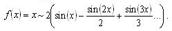 .
.
This is illustrated in Fig. 8, below.
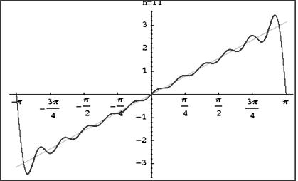
Fig. 8. The function y=x expressed as a sum of periodic functions
5.2. Spectral analysis and Kuznets, Kondratieff, and other Waves
The mathematical implication is that for any time series, a sequence of periodic functions may always be found that add up to approximate the original time series. The above mathematical fact does not, in and of itself, imply that there is any actual or other interpretation of this equivalence. In other words, the fact that there is a mathematical equivalence does not imply that there are real phenomena that exhibit the same characteristics. Nonetheless, it does not imply the reverse either, that is that there may be periodic behavior lurking behind some phenomena. In this case, Fourier analysis could be useful in teasing out the details.
Mankiw (2008) states flat out that there are no regularities in economic phenomena. Garrison (1989) states that Kondratieff waves are a product of ‘creative empiricism’ and equivalent to the fanciful shapes, for example, the head-and-shoulders or candle sticks, of technical stock traders – and have ‘no basis whatever in theory’. However, he later modifies this position to allow for wave-like phenomena that have some structural basis.
In fact, as we have shown above, economists have much reason to suspect that the latter is the case. They have long recognized periodic phenomena of both long and short periods. Business cycles are but one example, which are easily detected and found in data. Thus, it is not unreasonable to replicate the stylized facts of economic phenomena by suggesting that it is, in fact, the combination of a number of periodic phenomena. This has the advantage of reducing observable phenomena to other phenomena already explained.
Kondratieff waves, described in the previous sections, are cycles that alternate between periods of high growth, with rapid price rises, and periods of relatively slow growth, with falling prices. Regardless of the existence of the illustrated sequence of historical events, it remains controversial if there is, in fact, any fundamental periodic phenomenon of which these facts are manifest. However, recently, as we have outlined in the above sections, a number of researchers have found evidence for such waves.
A number of arguments against this include: (1) the fact that even though certain types of human events tend to recur, people learn from their mistakes and some expectations of cycles may smooth them out. Also, (2) the types of production and investment change over time, (3) long waves are hard to verify empirically, (3) we have shown (see Section 3) that there may be different mechanisms working for cyclical behavior at different time scales, and, lastly, (4) Fourier's theorem shows one can always find waves in any data set (even in a data set generated by random numbers).
Although Korotayev and Tsirel (2010) find evidence not only for Kondratieff waves, but also for Kuznets swings, Juglar cycles, and Kitchin cycles. Without going into too much detail, suffice to say that each of these periodic phenomena are characterized by different frequencies and amplitudes. Thus, it is no surprise (see argument 4 above) that analysis of data will show, with suitable adjustments/calibration, that the data series can be replicated by a sum of periodic functions.
Korotayev and Tsirel (2010) use spectral analysis in their research. They study world GDP growth rates and prices going back over 100 years. The particular form of spectral analysis they use is adapted to time-series. In this technique, the time-series is analyzed ‘based on the assumption that a broad class of aperiodic natural, technical, and social processes may be represented as sums of random process with stationary increments of different orders’. Now although this seems natural enough, and, in fact, given what we know about Fourier Series, must be mathematically true, the problem with the reasoning is this: we are assuming, in some sense, that what we want to find is already there; and then we go and find it. On the other hand, in any sort of modeling, one generally assumes some sort of structural relationship and then considers empirical data to see if there is evidence that supports it. Some might criticize the method of Korotayev and Tsirel because the period of the Kondratieff waves in their research has a period of around 50 years. Thus, no more than three complete cycles could exist in their database.
However, their approach is statistical, not a simple Fourier decomposition, and it has been shown that, even with such a small sample, the test statistic follows an x2 distribution. Thus, they obtain low p-values for those components with periods of approximately 50 years (Kondratieff waves; p = 0.04), periods of around 8 years (Juglar cycles, p = 0.025), and periods of close to 3.5 years (Kitchin waves, p = 0.025). With such p-values, most statisticians would accept the presence of these cycles. The key arguments regard the interpretation of historical economic and political events. Note that Korotayev and Tsirel prefer to regard Kuznets swings as harmonic elements of Kondratieff waves, rather than as a separate cycle.
5.3. Other methods of cycle detection
Another issue that comes up in Korotayev and Tsirel is the pre-processing of data. For example, in addition to eliminating the years of the two world wars, (1914–1919, 1939–1946), they also have ‘replaced all the values for the period between 1914 and 1946 with geometric means (1.5 % per year)’. This seems a rather extreme and arbitrary replacement. If cycles are to explain economic behavior, only limited adjustment of the data should be permitted. Further, in the second more radical departure from the actual data, ‘the values for years between 1914 and 1946 were replaced by the mean value (3.2 %) for the whole period under study (1871–2007), that is, those values were actually excluded from the spectral analysis’. Thus, it seems to bring into question as to what, in fact was being analyzed.
Additionally, we believe that a wiser course would have been to follow a more robust method of analysis – one that does not require such a large degree of pre-processing. For example, in Gallegati et al. (2011) a wavelet approach is used to determine the factors that effect output with considerations of size, scale, and time.
The key issue in the empirical analysis is the fact that there may be cycles of different times scales. This leaves open the possibility that they may amplify or counteract each other. For example, Kondratieff cycles in output and prices are estimated to have periods of around 45–60 years; Kuznets infrastructure cycles have periods of around 25 years; Schumpeter's ‘innovation’, 50 years, the Goodwin cycle of maybe 20 to 30 years, and Keynes–Kaldor–Kalecki cycles of demand: 7–9 years. Thus, the empirical analysis needs to be able to verify these cycles.
Wavelet analysis is similar to and sometimes more accurate than traditional spectral analysis because it uses short ‘wavelets’ instead of infinite periodic functions. In contrast to the Fourier analysis, wavelet analysis deals with the signal at varied frequencies with varied resolutions. Instead of the fixed time-frequency results of the Fourier analysis, the wavelet method provides excellent frequency resolution at low frequencies and good time resolution at high frequencies. Thus, this methodology allows both time and frequency to vary in time-frequency plane, but also the mechanisms driving those cycles.
In Gallegati et al. (2011), a wavelet approach was used to analyze the time series data underlying the Phillips curve.[10]
Thus, wavelets provide a good method to see relationships on different time scales and allow one to disentangle what drives output at different time horizons. Wavelet variance and cross-correlation methods can be used to determine leads and lags in time series and how different time scales affect them. This is likely to be a better approach to cyclical analysis of macroeconomic time series.
Yet another methodology for the decomposition and filtering of time series is the technique of penalized splines (see Kauermann et al. 2011). Here, a time-series is decomposed into a smooth path and a series of residuals, which are assumed to be stationary around the trend. This technique is robust with regard to correlation of residuals. The residuals exhibit business cycle features.
Splines are basically a type of smoothing, using basis functions, in which piece-wise polynomial functions are joined together to form a ‘smooth’ shape. Then the ‘smoothed’ shapes or periodicity and other features can be studied more easily than the original data-stream. In their paper, Kauermann et al. discuss several sub-methodologies including the Hodrick-Prescott (HP) Filter and the Bandpass (BP) Filter; these are contrasted with the method of penalized spline. They study GDP and its components from 1953 to 1996.
We see that there are a variety of approaches to the identification of cycles within time series methods. Each of them has some advantages and disadvantages.
5.4. Some empirics on the Goodwin cycle
Other analysis, for example, Flaschel et al. (2008) show how cyclical behavior can appear as Goodwin cycles, based upon predator-prey dynamics as discussed in Section 3.5. In their case, they show how, with suitable assumptions about the wage-price spiral and certain other variables, a Lotka-Voltera type of model gives rise to periodic phenomena, as explained in Section 3.5 above. In this case, the ambiguities are only pushed into the background, that is into the parameters and structure of the pair of differential equations that give rise to the dynamical system. In other words, it is not in question if the system they develop gives rise to periodic behavior, it does. The question is whether the system is well-grounded in the empirics of the variables being used.
At this point, we do not seek to advocate for or against the existence of wave-like phenomena in economic behavior. Instead, we only wish to point out two things: (1) Fourier's theorem guarantees that one can find a set of waves which fully simulate any curve; (2) there is a fundamental ambiguity about the nature of the economic behavior being explained with respect to frequency, amplitude, etc. as there is sufficient freedom for interpretation of virtually any periodic phenomena as ‘economic’ phenomena.
An empirical test of the cyclicality of synthesis of the Goodwin and Keynes-Kaldor models is given in Flaschel et al. (2008). Often the Goodwin model has been interpreted as business cycle dynamics, but as Flaschel et al. (2008) show, the employment and wage-share dynamics seems to hold more for a longer time scale, where the wage-share movement can be found to be related to a large time scale with a delay.
Employment seems to lead the change of the wage-share in the context of long waves (see Fig. 9).
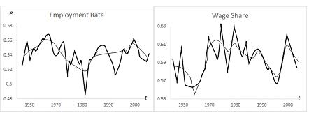
Fig. 9. U.S. Goodwin cycles
In examining business cycles, we note there is some negative correlation between employment and wage share. This interaction appears to come less from real wage movements, but rather from pro-cyclical productivity movements. As to the longer time scale – here captured by the thin solid trend line – as it is shown in Fig. 9, there seems to be a strongly delayed reaction. With employment rising, wage shares seem to rise with a delay, and as wage shares continue rising, employment seems to fall with a significant delay. Most of our current cycle models – on short or long scales – do not exhibit such delays.
5.5. Some empirics on the Minsky cycle
The period 1981–2007 provides evidence from the U.S. economy that is strongly supportive of the idea of a long Minsky cycle. The Minsky basic cycle embodies a sentiment-based theory of the business cycle (see also Semmler and Bernard 2012). The tranquil period generates increasingly greater risk taking as agents become progressively more optimistic. That optimism manifests itself in increasingly optimistic valuations of assets and associated revenue streams. It also manifests itself in credit markets where both borrowers and lenders become more optimistic. That is critical because it means lender-imposed market discipline becomes progressively weaker. Leveraging increases but the usual text-book scenario of corporate finance, whereby higher leverage implies a higher risk premium, is not visible in the cost of credit. Instead, credit remains cheap and plentiful.
Fig. 10 shows the ratio of home prices to rents during the period from the 1960s to 2006. Since 1999, the ratio suddenly starts to increase. Such a development would be consistent with a dramatic drop in interest rates, thereby generating a large increase in the present value of anticipated rents. However, that did not happen. Instead, the increase in home prices relative to rents was driven by speculative anticipations of higher resale values. This corresponds exactly with the Ponzi phase of the basic Minsky cycle in which agents borrow to finance asset purchases in anticipation of higher resale values.
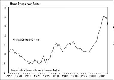
Fig. 10. Ratio of home prices: Rents
Fig. 11 shows nominal mortgage rates over the period 1971–2008. The figure shows that nominal mortgage rates rose sharply in the 1970s through to 1981, and then fell steadily through to 2002. Under ‘normal’ circumstances, it would be surprising to see a simultaneous increase of mortgage interest rates and the home price to rent ratio. However, the 1970s and early 1980s were a period of stagflation – rapid inflation plus relatively high unemployment. The rise in the home price to rent ratio can therefore be explained by the combination of increased demand for hard assets that are more protected against inflation and lowered rents attributable to a weak economy. With regard to the Minsky cycle, the main feature of interest in Fig. 11 is that mortgage interest rates remained roughly constant over the period 2002–2007. This was a period when the bubble in house prices had already set in and buying homes therefore involved larger mortgages.
Yet, despite this, there was no increase in risk premiums, reflecting the increased optimism and complacency of lenders.
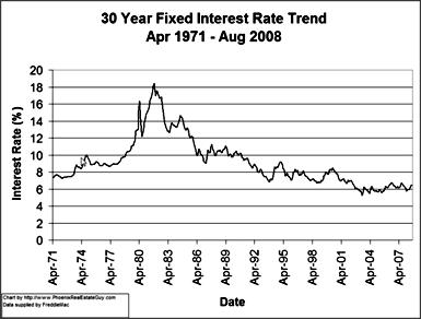
Fig. 11. Historical mortgage rates
Two further pieces of evidence consistent with the Minsky basic and super cycles are provided in Figs 12 and 13. Fig. 12 illustrates the percentage of disposable income devoted to servicing debt for the period 1980–2007. This is a fairly good proxy of risk since the lower the percentage of disposable income a borrower needs to pay (i.e. the lower the debt service burden), the less risky is the loan. Fig. 12 shows a cyclical pattern, with the debt service burden rising in the expansion of the 1980s and then falling when the economy went into recession. It rose again with the expansion of the 1990s, briefly flattened at the end of that expansion, and then continued increasing in the 2000s. This pattern is consistent with the interaction between the basic Minsky cycle and the Minsky super-cycle discussed earlier.
The basic cycle is evident in the expansions of the 1980s and 1990s, but by the 2000s the old thwarting institutions had been rendered obsolete and the economy enters a period of unsustainable boom that ends with a financial crisis.
During this last period, leverage increases massively but there is no increase in interest rate risk premiums because lender discipline was in tatters owing to the spread of optimism amongst lenders that weakened market discipline.
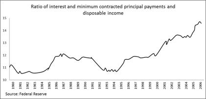
Fig. 12. Debt service to disposable income ratio
Fig. 13 shows the volume of funds in collateralized debt obligations (CDO) over the period 1992–2002. Collateralized debt obligations are financial assets constructed by bundling smaller loans. The interest and principal on these loans are paid to a trust entity, which then divides those payments among CDO owners. Distributions from the trust entity may also be tranched, with less risky CDOs receiving payment first and more risky CDOs receiving the remaining income. Mortgage-backed securities (MBS) represent a specific type of CDO backed by home mortgages.
As discussed earlier, an important ingredient of the Minsky super-cycle is financial innovation that escapes the regulatory net, permits increased risk-taking, and encourages financial complacency. CDOs represent such an innovation. The bundling of loans in CDOs enabled banks and other lenders to sell their loan portfolios and thereby off-load risk. This created the ‘originate and distribute’ model whereby banks and other lenders shifted to selling their loans rather than holding them. That in turn changed patterns of incentives, giving banks an incentive to push loans rather than engage in sound lending. That is because banks increasingly made money by taking the fees, commissions, and profits associated with creating CDOs and did not bear the ultimate risk associated with loan performance.
If the loan subsequently went bad it was no longer on the bank's book.
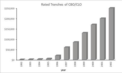
Fig. 13. Securitization of debt: Complex securities
The new CDO ‘originate and distribute’ lending model therefore relaxed lender discipline since lenders felt they were not ultimately on the line. This helps explain why debt service burdens were allowed to increase so much and why interest rates did not rise to reflect increased risk premiums. On a global scale, proliferation of such ‘robust’ new financial instruments invokes the redefined fundamental uncertainty framework (Gevorkyan and Gevorkyan 2012). With unclear recovery prospects as investors, driven by portfolio maximizing strategies, pour in and abruptly exit the emerging financial markets, the full brunt of the recent crisis is yet to unravel in the structurally weaker economies.
6. Conclusion
Empirically detecting the mechanisms of long cycles is difficult. First, there are technical challenges associated with filtering and spectral methods. Second, and more important, economies are characterized by continuous change that becomes ever more significant as the period of analysis lengthens. For instance, Kuznets and Kondratieff waves of twenty-five to fifty year duration will inevitably take place in a context of significant structural change. Over the last two hundred years, a repeated sequence of structural change has been the transformation of economic activity from agricultural dominance to manufacturing dominance, then on to service sector dominance. Economies are also characterized by institutional change concerning labor markets, regulatory arrangements, and the organization of firms.
These institutional changes alter the processes of decision-making, introduce new decision actors and interest groups, and change the balance between market and government. Technological change has promoted a trend to economic activity that involves less physical production and resource use, and is more intensive regarding knowledge based production activity. As a result, the character and forces of growth are likely to change.[11] From that perspective, one can never step in the same river twice.
The existence of so much historically idiosyncratic matter makes it empirically difficult to detect cycles of fixed periodicity and amplitude based on time invariant cycle generating mechanisms. Wavelet methods appear to be the most suitable means of empirically identifying economic relationships over cycles of different duration. Technical difficulties notwithstanding the data for some macroeconomic variables (particularly profits) exhibit the dynamics of ups and downs. It also appears possible to talk about stages, or phases, regarding the economic dynamics of developed and emerging market economies. If long cycle theory holds, that raises the question of where we stand today. Are we in the middle of a cycle or at the end of one and awaiting the beginning of another? Those are the questions that the application of long cycle theory and methods may help answer.
References
Akaev A. A. 2009. The Current Financial and Economic Crisis in the Context of the Theory of Innovative Technological Development of Economy and Control over Innovative Process. System Monitoring. Global and Regional Development / Ed. by D. A. Khaltourina, and A. V. Korotayev, pp. 141–162. Moscow: URSS. In Russian (Акаев А. А. Современный финансово-экономический кризис в свете теории инновационно-технологического развития экономики и управления инновационным процессом. Системный мониторинг. Глобальное и региональное развитие / Ред. Д. А. Халтурина, А. В. Коротаев, с. 141–162. М.: УРСС).
Bernanke B. 2004. The Great Moderation. Remarks at the Meetings of the Eastern Economic Association. Washington, DC, February 20. URL: http://www.federal reserve.gov/boarddocs/speeches/2004/20040220/
Bernanke B., Gertler M., and Gilchrist S. 1996. The Financial Accelerator and the Flight to Quality. Review of Economics and Statistics 78: 1–15.
Bernanke B., Gertler M., and Gilchrist S. 1999. The Financial Accelerator in a Quantitative Business Cycle Framework. Handbook of Macroeconomics. Vol. 1 / Ed. by J. B. Taylor, and M. Woodford, pp. 1341–1393. Amsterdam – New York – Oxford: Elsevier Science.
Buniatian M. A. 1915. Economic Crises. Morphology, Theory of Periodical Economic Crises and Theory of Market Conditions. Moscow: Mysl. In Russian (Бунятян М. А. Экономические кризисы. Опыт морфологии и теории периодических экономических кризисов и теории конъюнктуры. М.: Мысль).
Chang W., and Smyth D. L. 1971. The Existence and Persistence of Cycles in a Non-Linear Model: Kaldor's 1940 Model Re-Examined. Review of Economic Studies 38: 37–46.
Delli Gatti D., Gallegati M., and Minsky H. 1994. Financial Institutions, Economic Policy, and the Dynamic Behavior of the Economy. Working Paper No. 126. New York: The Jerome Levy Economics Institute of Bard College.
Ferri P., and Minsky H. 1992. Market Processes and Thwarting Systems. Structural Change and Economic Dynamics 3: 79–91.
Flaschel P. 1984. Some Stability Properties of Goodwin's Growth Cycles. Zeitschrift fur Nationaloekonomie 44: 281–285.
Flaschel P., and Semmler W. 1987. Classical and Neoclassical Competitive Adjustment Process. Manchester School of Economic and Social Studies 55(1): 13–37.
Flaschel P., Tavani D., Taylor L., and Teuber T. 2008. Demand Driven Goodwin Growth Cycles with a Three-Regimes Wage Phillips Curve. Working Paper No. 153. University of Bielefeld: Center for Empirical Macro- and Microeconomics.
Gallegati M., Ramsey J., and Semmler W. 2011. Forecasting Output Using Interest Rate Spreads: A Wavelet Decomposition Analysis. (In Press.)
Gallegati M., Gallegati M., Ramsey J., and Semmler W. 2011. The US Wage Phillips Curve Across Frequencies and Over Time. Oxford Bulletin of Economics and Statistics 73(4): 489–508.
Garrison R. 1989. The Austrian Theory of the Business Cycle in the Light of Modern Macroeconomics. Review of Austrian Economics 3: 3–29.
Garvy G. 1943. Kondratieff's Theory of Long Cycles. The Review of Economics and Statistics 25(4): 203–220.
Van Gelderen J. 1913. Springvloed: Beschouwingen over industrieele ontwikkeling en prijsbeweging (Spring Tides of Industrial Development and Price Movements). De nieuwe tijd 18.
Gevorkyan A. V. 2011. Innovative Fiscal Policy and Economic Development in Transition Economies. Oxford, UK: Routledge.
Gevorkyan A. V., and Gevorkyan Ar. 2012. Redefined Fundamental Uncertainty, Fiscal Rules, Fiscal Net, Fiscal Sustainability and Emerging Markets Scenarios. Aestimatio, the IEB International Journal of Finance 5: 126–161.
Goodwin R. 1967. A Growth Cycle. Socialism, Capitalism and Economic Growth / Ed. by C. H. Feinstein, pp. 54–58. Cambridge: Cambridge University Press.
Greiner A., Semmler W., and Gong G. 2005. The Forces of Economic Growth. Princeton, NJ: Princeton University Press.
Grossman G. M., and Krueger A. B. 1995. Economic Growth and the Environment. Quarterly Journal of Economics 110: 353–377.
Guckenheimer J., and Holmes P. 1983. Nonlinear Oscillations. Dynamical Systems and Bifurcations of Vector Fields. Berlin – New York: Springer.
Hicks J. R. 1950. A Contribution to the Theory of the Trade Cycle. Oxford, UK: Clarendon Press.
Hirsch M. W., and Smale S. 1974. Differential Equations, Dynamical Systems and Linear Algebra. New York: Academic Press.
Ito T. 1978. A Note on the Positivity Constraint in Olech's Theorem. Journal of Economic Theory 17: 312–318.
Juglar C. 1862. Des Crises commerciales et leur retour periodique en France, en Angleterre,et aux Etats-Unis. Paris: Guillaumin.
Kauermann G., Krivobokova T., and Semmler W. 2011. Filtering Time Series with Penalized Splines. Studies in Nonlinear Dynamics and Econometrics 15(2). DOI: 10.2202/1558-3708.1789.
Kaldor N. 1940. A Model of the Trade Cycle. Economic Journal 50: 78–92.
Kaldor N. 1971. A Comment. Review of Economic Studies 38: 45–46.
Kalecki M. 1937. A Theory of the Business Cycle. Review of Economic Studies 4: 77–97.
Kalecki M. 1971. Selected Essays on the Dynamics of the Capitalist Economy. Cambridge, UK: Cambridge University Press.
Kitchin J. 1923. Cycles and Trends in Economic Factors. Review of Economics and Statistics 5(1): 10–16.
Kiyotaki N., and Moore J. 1997. Credit Cycles. Journal of Political Economy 105: 211–248.
Kondratieff N. 1935. The Long Waves in Economic Life. Review of Economics and Statistics 18(6): 105–15.
Kondratieff N. 2002. Big Cycles of Conjuncture and Theory of Prevision: Selected Works / Ed. by Y. V. Yakovets, and L. I. Abalkin. In Russian (Кондратьев Н. Д. Большие циклы конъюнктуры и теория предвидения. Избранные труды / Pед. Я. В. Яковец, Л. И. Абалкин. М.: Экономика).
Kondratieff N. 2004 [1922]. The World Economy and its Conjunctures During and After the War / Ed. by Y. V. Yakovets, and N. A. Makasheva; transl. by V. Wolfson. Moscow: International Kondratieff Foundation.
Korotayev A., and Tsirel S. 2010. A Spectral Analysis of World GDP Dynamics: Kondratieff Waves, Kuznets Swings, Juglar and Kitchin Cycles in Global Economic Development, and the 2008–2009 Economic Crisis. Structure and Dynamics 4(1). URL: http://www.escholarship.org/uc/item/9jv108xp
Kuznets S. 1934. National Income, 1929–1932. U.S. Senate document no. 124, 73rd Congress, 2nd session.
Kuznets S. 1937. National Income and Capital Formation, 1919–1935. New York: National Bureau of Economic Research.
Kuznets S. 1949. National Income and Industrial Structure. Econometrica 17: 205–241.
Kuznets S. 1955. Economic Growth and Income Inequality. The American Economic Review 45(1): 1–28.
Kuznets S. 1965. Economic Growth and Structure: Selected Essays. New York: Norton.
Kuznets S. 1966. Modern Economic Growth: Rate, Structure, and Spread. New Haven, CT: Yale University Press.
Kuznets S. 1971. Economic Growth of Nations: Total Output and Production Structure. Cambridge, UK: Belknap Press of Harvard University Press.
Kuznets S. 1973. Modern Economic Growth: Findings and Reflections. The American Economic Review 63(3): 247–258.
Mankiw N. 2008. Principles of Economics. 5th ed. Mason, OH: South-Western.
Marx K. 2003 [1867]. Capital: A Critique of Political Economy. Vol. I. The Process of Capitalist Production. New York: International Publishers.
Minorsky N. 1962. Nonlinear Oscillations. New York: D. Van Nostrand Co.
Minsky H. P. 1957. Monetary Systems and Accelerator Models. American Economic Review 47: 859–883.
Minsky H. P. 1959. A Linear Model of Cyclical Growth. Review of Economics and Statistics 41: 133–145.
Minsky H. P. 1983. Financial Structure, Indebtedness and Credit. Paper prepared for an International Colloquium ‘Keynes Today: Theories and Policies’. September, 12. University of Paris I. Pantheon-Sorbonne.
Minsky H. P. 1992a. The Financial Instability Hypothesis. Working Paper No. 74. New York: The Jerome Levy Economics Institute of Bard College.
Minsky H. P. 1992b. Schumpeter and Finance. Market and Institutions in Economic Development: Essays in Honor of Paulo Sylos Labini / Ed. by S. Biasco, A. Roncagia, and M Salvati, pp. 103–115. New York: Macmillan Press.
Palley T. I. 2010. The Limits of Minsky's Financial Instability Hypothesis as an Explanation of the Crisis. Monthly Review 61(11): 28–43.
Palley T. I. 2011. A Theory of Minsky Super-Cycles and Financial Crises. Contributions to Political Economy 30(1): 31–46.
Reati A., and Toporowski J. 2004. An Economic Policy for the Fifth Long Wave. BNL Quarterly Review 57(231): 395–437.
Rostow W. W. 1975. Kondratieff, Schumpeter, and Kuznets: Trend Periods Revisited. The Journal of Economic History 35(4): 719–753.
Samuelson P. A. 1939. Interactions between the Multiplier Analysis and the Principle of Acceleration. The Review of Economic and Statistics 21: 75–78.
Schumpeter J. A. 1939. Business Cycles: A Theoretical, Historical and Statistical Analysis of the Capitalist Process. New York: McGraw-Hill.
Schumpeter J. A. 1970. Capitalism, Socialism and Democracy. New York: Harper & Row.
Schumpeter J. A. 2007 [1934]. The Theory of Economic Development. New Brunswick, NJ: Transaction Publishers.
Semmler W. 1986. On Nonlinear Theories of Economic Cycles and the Persistence of Business Cycles. Mathematical Social Sciences, Elsevier-North Holland 12: 47–76.
Semmler W., and Bernard L. 2012. Boom-Bust Cycles: Leveraging, Complex Securities, and Asset Prices. Journal of Economic Behavior and Organization 81(2): 442–465.
Stern D. I. 2004. The Environmental Kuznets Curve. International Encyclopedia of Ecological Economists. URL: http://www.ecoeco.org/pdf/stern.pdf
Tolstov G. 1962. Fourier Series. New York: Dover.
Velupillai K. 1979. Some Stability Properties of Goodwin's Growth Cycle. Zeitschrift fur Nationalokonomie 39: 245–257.
Whalen C. J. 1999. Hyman Minsky's Theory of Capitalist Development. Working Paper No. 277. New York: The Jerome Levy Economics Institute of Bard College.
De Wolff S. 1924. Prosperitats- und Depressionsperioden. Der Lebendige Marxismus / Hrsg. O. Jenssen, S. 13–43. Jena: Thuringer Verlagsanstalt.
World Bank (WB). 1992. World Development Report. Washington: The World Bank.
Wray L. R. 2009. Money Manager Capitalism and the Global Financial Crisis. Macroeconomic Policies on Shaky Foundations: Whither Mainstream Economics? / Ed. by E. Hein, T. Niechoj, and E. Stockhammer, pp. 283–306. Marburg: Metropolis-Verlag.
[1] See Juglar 1862.
[2] A review of the mechanisms of cycles on a shorter time scale is given in Semmler (1986).
[3] For details see Reati and Toporowski (2004).
[4] For details of the subsequent dynamic modeling see Semmler 1986.
[5] This conversion seems permissible as long as there are no savings out of workers income and thus workers income is completely spent for consumption. This is what Kalecki assumes.
[6] The curve is downward or upward sloping when (or ). By assuming that for a certain region , is upward sloping and also has a positive but steeper slope, it follows that there is only one unique equilibrium point. For similar assumptions concerning an income/investment model, see Chang and Smyth (1971: 40).
[7] A proof using the Poincare–Bendixson theorem is given in Semmler (1986).
[8] In a monetary economy, a very important factor effecting the change of signs in seems to be the financial condition of firms and the banking system (see Minsky 1983).
[9] On the usefulness of wavelets to study cycles at different time scales see Gallegati, Ramsey and Semmler (2011).
[10] Note that Goodwin uses such a Phillips curve but assumes a constant productivity growth rate and real variables.
[11] Greiner, Semmler and Gong (2005) show how modern growth involves more copying from others, combined with build-up of education and human capital, infrastructure, and knowledge creation.