The Paradigm Shift Cycle as the Cause of the Kondratieff Wave

Almanac: Kondratieff waves:Processes, Cycles, Triggers, and Technological Paradigms
DOI: https://doi.org/10.30884/978-5-7057-6191-3_03
Paradigm shifts in physics happen at 80-year intervals due to two constraints on physics and technology development that constrained the duration of paradigm development to average 80 years. These two constraints cause three generations to produce a physics paradigm and begin the industrialization during an industrial revolution. During each industrial revolution, there is a depressionary era due to the low productivity growth of the dying industries and the transition of the economy to new industries. Another depressionary era begins about 30 years after the end of the depressionary period of the industrial revolution. These depressions are times of high productivity growth when the industries reach the mature stage. The switch of emphasis from product innovation to process innovation causes depressionary eras during which the high corporate and consumer debt, product satiation, oligopoly formation, and increased automation that reduces the demand for labor cause depressions. The duration of the Kondratieff waves varies from about 40 to about 53 years depending on how quickly a paradigm is accepted.
Keywords: paradigm shifts in physics, scientific revolutions, industrial revolution, paradigm shift cycle, long wave cycle, economic long wave, Kondratieff waves, technological revolution, economic depression, technological acceleration, productivity growth acceleration, automation, unemployment, crisis periods, product innovation, process innovation, automation, labor displacement, physics paradigms.
Introduction
Nikolai Kondratieff among other scholars of the first half of the 20th century believed that the Kondratieff cycle had duration of about half a century because they only had the data from the 19th and late 18th centuries available to make this estimation. But since then, a 40-year timing instead of a half-century timing is seen to better fit the data. Economic growth depends largely on technological advancement that is driven by the advancement of physics. The cycle of paradigm shifts in physics involves the introduction of new paradigms by revolutionary scientists and has frequency of 80 years. It causes the economic long wave so that there is a depressionary trough and upswing during each scientific and industrial revolution era when the productivity growth is very low and a different kind of depressionary era characterized by accelerating productivity growth midway between the scientific and industrial revolutions.
The duration of an economic long wave depends on several factors. The main factor is how rapidly a society accepts a new paradigm of physics. If they accept the paradigm quickly as happened in the last half of the 1700s, then the two long waves that follow after may be longer as happened in the 1800s. As described in this paper, the rapid spread and acceptance by society of the fluid paradigm during the middle of the 1700s caused rapid development of technology of the fluid paradigm in the late 1700s so that within about four decades from the introduction of some very basic ideas of the fluid paradigm in 1745, scientists and engineers who understood the paradigm began to build significant industries in Britain. This was the First Industrial Revolution of the late 1700s.
In contrast, during the 19th century, the scientists and the people in general accepted the physics ideas of Faraday involving point atoms and lines of force relatively more slowly, so the Second Industrial Revolution that started about 1880 lagged the introduction of the classical field theory paradigm in 1820 by about 60 years. This is why the period of time from the beginning of the first upswing of the first long wave about the year 1800 to the beginning of the upswing of the third long wave in 1900 in the US was about 100 years so that the first two long waves were about 50 years in length instead of 40 years.
The 40-year cycle frequency for the Kondratieff wave fits better with the economic data for the 20th and current centuries. A severe depression period started about 1930, the deepest recession period of the 20th century about 1970, and it is clear that the stage was set in 2008 for another depression or long-lasting severe recession. However, most of the last 13 years has not been a deep recession or depression per se because for the first time during a Kondratieff trough, unprecedented debt creation during a time of peace kept the economy from contracting. About US$ 22 trillion dollars of US deficit spending and stimulus measures from the 2008 stock market crash through the fall of 2022 have so far kept the consumers from experiencing severe hardships. Other countries have also been stimulating their economies with very large deficit financing. Extra tens of trillions of debt creation may not be enough to keep the economy from experiencing a contraction and the associated effects of this kind of depression that happens between industrial revolutions.
The Paradigm Change Cycle
Physics paradigms develop through three necessary stages. According to Kuhn (1970), a young, inexperienced person, aware of unresolved stark anomalies of a 10- or 20-year long crisis period, conceives new basic physics hypotheses quite different than those of the older paradigms and teaches his theory. Then the basic theory needs to be elaborated, developed, and mathematically described. Then the elaborated and well-defined theory is tested experimentally, and major anomalies are again discovered during another 10- or 20-year long physics crisis period.
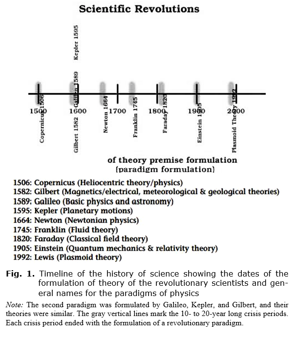
In the history of the development of science since 1500, each of these three stages of development of a paradigm has been achieved by each successive generation to create an 80-year period of three stages of about 27 years each. To produce a mature physics paradigm through the stages of theory formulation, theory development, and experimentation that produces both validating and anomalous phenomena, three generations are required. The first generation formulates the basic premise of the paradigm, the second generation develops the theory, and the third one performs the crucial experiments. The consistency of this 80-year timing is remarkable. In the timeline in Fig. 1, the duration between instances of paradigm formulation varies from about 73 to 87 years.
Two Major Constraints on Paradigm Development
There are two main reasons for this paradigm development pattern that I call the Constraint of Inhibition of Apprehension and the Constraint of the Difference Between Theoreticians and Experimenters. These two social constraints make paradigm development happen over three generations. The first reason that delays full theoretical development of a new paradigm until the second generation is that the formulator of a paradigm has not been able to develop his theory sufficiently, and almost no one of his generation understands his basic concepts implicitly. The reason for this is that by the time the formulator conceptualizes and sufficiently develops and publishes his ideas, those of his own generation are too old and too experienced with the prior paradigm to believe or well understand his ideas. Their experience and training in an older paradigm inhibits their apprehension of the new paradigm. I call this first reason the Constraint of Inhibition of Apprehension. Thomas Kuhn described this constraint by saying that the young and inexperienced are the paradigm formulators. Conversely, age and prior experience in a prior paradigm makes people unable to well accept and develop new paradigms.
A few years after the first formulation, after the formulator publishes his ideas, some part of the society may accept his ideas. Then, younger theoreticians in the next generation who believe the basic ideas of the new paradigm develop the theories of the paradigm. Generally, this stage of theoretical development is completed about 40 years after the date of the first conception of the paradigm.
A case in point is that of the quantum mechanics and relativity paradigm. It is generally acknowledged that quantum mechanics was well developed by about 1948 when Tomonaga, Schwinger, and Feynman had more or less independently finished the development of the theory of quantum electrodynamics for which the three physicists received the Nobel Prize in 1948. All three of these men were born within 13 years of the first formulation of the basic ideas of the quantum mechanics paradigm by Einstein in 1905. They were among the generation of theoretical developers. Thus, the development of quantum mechanics theory was finished by about 43 years of the time its basic ideas were first formulated. The three developers of QED theory are examples of the second generation of theorists who completed development of a major theory of the paradigm. The gravitational aspects of the 20th-century paradigm were mainly completed before the 1940s by Einstein so that by the middle of the 1940s, both major branches of the Einstein quantum mechanics and relativity paradigm were well developed.
Then, during the crisis periods starting about 60 years after the first formulation, the members of the third generation of the society accomplished their experimental work of discovering anomalies. Kuhn wrote that these periods gene-rally last from 10 to 20 years (Kuhn 1970). The last four crisis periods occurred from 1725 to 1745, 1800 to 1820, 1880 to 1905, and 1972 to 1992.
A crisis period happened between 1725 and 1745. At this time, Martine discovered anomalies to the Newtonian theory of heat, and two experimenters invented the Leyden Jar, the condenser for electricity, that allowed Franklin to perform groundbreaking experiments in 1745 and afterwards. Martine and the inventors of the Leyden jar were among the third-generation experimenters of the paradigm who produced the crucial anomalous phenomena.
Another crisis period happened from about 1800 to 1820. At that period Davy discovered anomalies to the Fluid theory of heat, and Oersted discovered the electromagnetic effect that contradicted the basic hypotheses in the Franklin paradigm that these were two different fluids. The third crisis period happened from 1880 to 1905 during which time experimenters discovered major anomalies including particles, the quantum effect, and the evidence pointing to the invariance of the speed of light. The fourth crisis period lasted from the early 1970s to 1992. At that time, experimenters discovered major anomalous phenomena such as the existence of plasmoids, their long existence in matter, anomalous energy concentration, and the creation of microplasmoids associated with transmutation effects (for more details see below).
However, up till the present time, the theoretical developers and those of their generation have not been able to experimentally find the anomalies of the developed theories. For example, one can see that the necessary technology for the discovery of the major anomalies of the fluid paradigm and field theory paradigm was not available during the 1780s and the 1940s when the theories of the two paradigms became developed. The necessary technology and experimental apparatus were developed about 20 years afterwards. So they could not perform the experiments that the next generation of experimental researchers performed in the crisis periods after 1800 and after 1970. For example, the battery used to produce the electromagnetic effect was not invented until 1800. This effect was one of the major anomalous phenomena that allowed Faraday and others to develop classical field theory and electromagnetic technology. Likewise, scanning electron microscopes that have been used for both microscopic examination of features of a sample and for analyzing chemical composition at small scales became commercially available about the year 1965. It has been a principle tool for discovering microplasmoids and their effects.
The reason for this approximately 60-year delay between formulation of the basic principles of a physics paradigm and the start of a crisis period seems to be the general principle that experimentally skilled scientists and inventors must first grow up believing a paradigm and being trained to utilize it well since their youths. As the consequence of the Constraint of Inhibition of Apprehension, only younger people can implicitly apprehend the basic theory a formulator teaches. The theorists of the second generation also generally do not possess necessary technical skills. Thomas Kuhn also described this difference between theoreticians and experimenters in his book (see Kuhn 1970). I call the second constraint the Constraint of the Difference Between Theorists and Experimenters for lack of a better name. Thus, because of the two constraints on physics development, the work of creating and performing experiments that can discover the crucial anomalies is done during the crisis period by the third-generation of experimenters who had grown up being trained in the paradigm. It is then that the necessary technology becomes available and the experimenters develop a high level of competence for their research.
At the end of each crisis period, the formulator of a new paradigm conceives new postulates of physics based on the evidence of the anomalies. In most of the cases except Franklin and Gilbert, the formulating physicist was young and inexperienced. But Franklin and Gilbert were both middle-aged. Franklin was in his middle age when he formulated his basic fluid ideas in 1745 that were based in part on the just discovered Leyden jar effect. Franklin was chronologically older, but he was inquisitive and relatively inexperienced as a scientist. So he was able to make his conceptual leaps because he did not try to interpret the new electrical and heat anomalies according to the older paradigms of the era, but he approached the effects with a fresh mind.
Overall, these three generations have accomplished their
work of performing these three stages of paradigm development within an approximately
80-year period.
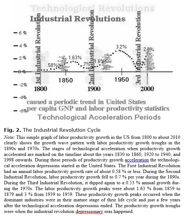
Each physics paradigm enables the advance of technology. Each of the three industrial revolutions had inventions of new power sources. In the case of the Franklin paradigm, the theory of the fluid of heat enabled the invention of the steam engine by Watt that was a great new source of motive power. The fluid or caloric chemistry also allowed for the production of some important industrial chemicals. The economic effect of the technological innovation was revolutionary. So productivity grew in a curvilinear fashion as I plotted in Fig. 2 for the US. The productivity growth in Britain during the 19th century mirrored this, but their labor productivity growth curve was ahead of the US by about 10 or 15 years since it was the technological leader of the fluid paradigm. The US was the technological follower throughout most of the 19th century.
The technological innovation cycle has three general stages. The first stage is that of industrial revolution involving the inception of major industries with an emphasis on product innovation. The second stage that begins about 20 years after the end of an industrial revolution depressionary era is the switch from the emphasis on inventing new kinds of products to process innovation. At this stage, companies compete for market share on standardized products by emphasizing automation of their production. They try to utilize economies of scale and automation to reduce the cost of production. Corporations and firms amass debt, and there is a huge increase of mergers and acquisitions. When industries did this during the last three paradigms, they laid off a large number of their workers. The displacement of human labor caused a decrease in consumption for the standardized products of industry starting about the years 1830, 1929, and 2008. There was also a satiation of demand for the available products of industries. The drop of consumption and unemployment caused the financial crises of the past three paradigms and depressionary eras.
The third stage is the senescence and death phase of the industrial life cycle. Simon Kuznets showed how toward the end of the 1800s, a number of major industries of that era experienced both a dearth of innovation and death as they were replaced by newer industries based on electricity, petrochemicals, and the internal combustion engine (Kuznets 1930). During this time of industrial revolution and the death of the old industries at the end of the 19th century, labor productivity growth dropped to a secular historical low in both the US and Britain. The same thing happened to the industries based on the classical field theory in the 1960s and 1970s. By the late 1960s, the big dominant industries of that time such as the automobile, telephone, and steel industries had a marked lack of innovation and exhibited almost zero productivity growth around the year 1970, and the productivity growth dropped to the lows experienced in the US of the 1970s and early 1980s (see Fig. 2).
These three stages of the industrial revolution cycle happen during three or four generations. Unlike the three stages of scientific revolution and paradigm development, the three-stage process of industrial development and death is less precisely three generations. In part, this is because the time between industrial revolutions is less precise. As explained, the duration of the inception, development, and replacement of paradigm industries depends in part on how quickly society accepts a new scientific paradigm. There were 100 years between the First Industrial Revolution and the Second Industrial Revolution and 82 years between the Second Industrial Revolution and the Third Industrial Revolution. This is calculated by dating from the end of the depressionary eras associated with the industrial revolutions.
The Labor Productivity Statistics in the US
Statistics for labor productivity growth and the annual growth rate of real per capita GDP in the US economy from 1800 to 1997 compiled by economists such as Paul Romer shows this curvilinear trend of productivity growth with an 80- to 90-year periodicity. According to Paul Romer, average per capita growth of GDP was 0.58 % per year during the period 1800–1840[1] (Romer 1985). The statistics for labor productivity at this early date may yet be unavailable. Labor productivity increased about 1.3 % per year on average during the period of 1839–1859. From 1859 to 1879, it increased about 1.4 % per year when US labor productivity growth peaked. In the period from 1879 to 1899, it increased only about 0.7 % annually during the depression caused by the transition to new paradigm industries and the depletion of the potential of the older kind of technology that was based on the fluid paradigm.
Then it increased to about 1.6 % in 1899–1919 and about 2.2 % in 1919–1939. It rose to a peak of 3.0 % per year during the period of 1939 to 1959. It again decreased to about 2 % per year during the period of 1959 to 1979[2] (Romer 1989). In 1973–1981, during another conjuncture and the deepest recession period of the 20th century, American labor productivity dipped to about 1 % per year in another major trough. Then from 1982 until the 2008 crash, the US labor productivity increased about 2 % per year or so. Labor productivity growth doubled about the year 1998.
It reached a high of about 3 % in 2010 as the deep recession after the crash happened as one would expect according to this theory. During the 1930s, due to the increased unemployment and the extensive implementation of automation, labor productivity growth kept rising. Since 2010, however, labor productivity in the United States has actually decreased. But I believe that this is due to about US$ 6 trillion dollars of national debt added in the USA alone from 2008 to 2012 plus more than a trillion US dollars every year until the current epidemic began in 2020. This helped the millions of U.S. consumers to avoid the extreme poverty of the 1930s and maintain a level of standard of living and level of consumption not based on production but on borrowing.
Americans are heavily in debt. In the fall of 2022, US corporate debt is about US$ 50 trillion dollars. The US household consumer debt passed US$ 16 trillion in 2022. Due to the national, consumer, and corporate debt, wages and employment remained high during the 2010s and labor productivity decreased. However, during the similar depression periods that began in 1830 and 1929, without comparable governmental stimulus and intervention, the rapid automation and the great increase of unemployment enabled the high labor productivity growth rates that started in Britain in the 1820s and the United states in the 1920s to continue to increase to the highs recorded in the US of 1.4 % per year during the period of 1859 to 1879 and 3.0 % per year in 1939 –1959.
Overall, the historical lows of labor productivity coincided with the industrial revolutions. That is, in the United States, it was a low of about 0.58 % or below in the early 1800s, a low of about 0.53 % in the 1890s, and a low of about 1 % from 1973 to 1981. For the First Industrial Revolution, the Second Industrial Revolution and the Third Industrial Revolution, there was a doubling of labor productivity growth rates about 20 years after the end of the depressionary eras that ended in 1800, 1900, and 1982. In 1820 in Britain and in 1920 and 1998 in the United States, labor productivity growth suddenly doubled.
Paul Waters noticed the doubling of productivity growth in the USA in 1920, and he called the event a technological acceleration (Waters 1972[1977]).
The Causes of the Technological Acceleration Induced Depressions
In his book, Technological Acceleration and the Great Depression, Waters tried to explain how the sudden increase of productivity associated with a massive increase of consumer credit that was made available during the 1920s caused the Great Depression (Ibid.). His book was insightful. But he did not take into consideration the effect of automation and greater economies of scale of the conglomerate oligopolies that formed in the 1920s on causing unemployment to increase. He also did not describe the effect of satiation of demand for standardized products. Waters focused on the financial and debt situation in the U.S. economy.
During the middle stage of the industrial life cycle when industries had switched their focus from product innovation to process innovation, the same depressionary causes existed during the three industrial revolutions. In the 1820s, 1920s, and in the first decade of the 2000s, there were the same characteristics of rising productivity due to the displacement of labor by automation, oligopoly formation and higher efficiencies of scale, increasing business and consumer debt, and the satiation of consumer demand of the available types of products within the constraints of their budgets. These four causes caused the technological acceleration depression eras that started in 1830, 1929, and 2008.
Two Types of Kondratieff Long Wave Troughs
From the above analysis, one can see that the 80-year cycle of paradigm shifts produces two different kinds of long wave troughs. The depressionary eras associated with industrial revolutions occur as economies transition between the industries of two paradigms. The industrial revolutions and paradigm shifts approximately coincide. It depends on how relatively quickly the paradigms develop.
The other type of depressionary era happens in the middle of the industrial revolutions, generally about 30 years after the end of the depressions associated with industrial revolutions. I call these depressions technological acceleration depressions that happen during the middle stage of the industrial life cycle when industries transition from product innovation to process innovation. The rise of automation, as is happening now in industry and business, raises the unemployment. These types of depressions have been more severe. Currently, more than US$ 22 trillion dollars of added national debt in only the past 14 years since the 2008 financial crash, the stimulus spending, and the government subsidies are preventing severe depressionary contraction. Thus, this shows that this Kondratieff wave model is correct.
The Three Paradigms (1500–1745)
In 1506, Copernicus formulated a paradigm for physics and astronomy according to which impetus was assumed to be the reason that things did not fall off the round and moving planet. This basic assumption was an important postulate of his theory. His theory was developed after him by other astronomers of the next generation, and after that in the third generation, some experimenters and astronomers started finding important new physical anomalies and astronomical phenomena that contradicted his heliocentric model.
Then, Gilbert, Galileo and Kepler (in 1582, 1593, and 1595 respectively) coincidentally but more or less independently of each other thought that fall was a magnetic effect. Thus, they believed that gravity is magnetism. Both Galileo and Kepler had read the scientific texts of Gilbert, so their theoretical work was not entirely independent of his theory. They also believed that bodies had a tendency to rest that contrasts with the important and fundamental concept of inertia introduced by Newton. Again, a second generation of scientists developed paradigm theory mathematically and conceptually. Among these were Descartes and many others. Then, in the third generation, experimenters discovered crucial physical anomalies.
Then Newton discovered gravity in 1664. He thought that corpuscular atoms have the invisible force of gravity. He developed the theories of the paradigm substantially by himself. He taught other English people about phenomena, and he worked strenuously to make sure that his theory of phenomena was accepted by people and taught to the next generation. Through his work, most of the English either accepted or apprehended a theory similar to his by the early 1700s. Educated people such as Voltaire noticed a stark difference between the physics believed by the English and that believed by the French. The French and others on the Continent continued to develop and teach theories similar to those of Galileo and Descartes during the early 1700s while the English developed the Newtonian paradigm.
Starting about 1725, a third generation of experimenters discovered anomalies. Martine detected heat anomalies in 1741. Then in 1745, van Musschenbroek and von Kleist independently invented the anomalous Leyden jar to store electricity generated from a machine invented by Hauksbee. Living on the Continent, they seem to have believed the theories of the prior Galileo and Descartes' paradigm. But Hauksbee was an Englishman who was a student of Newton. George Martine was born and educated in Scotland where the Newtonian paradigm was accepted. He was born in 1700, so he was in the third generation after Newton.
The Three Paradigms and the Three Industrial
Revolutions from 1745 Onwards
For understanding the Kondratieff long wave which, according to Kondratieff, began during the First Industrial Revolution of the late 1700s, it is necessary to study how the three paradigms of fluid theory, field theory, and quantum mechanics and relativity theory were used to develop the industries of the three revolutions.
The Development and Rapid Acceptance of the Franklin Paradigm
About the year 1745, Franklin conceived hypotheses about conserved fluids for heat and electricity, and he may have introduced the hypothesis of the magnetic fluid at this time or later. His model of the Universe in which fluids of heat, electricity, and magnetism moved and flowed and were conserved was revolutionary.
Franklin wrote highly influential articles and books. Quite quickly in comparison to the other revolutionary researchers, by the mid-1750s, he became a world-famous scholar. He is well-known worldwide for proving that lightning was electricity, and his general popularity and political fame spurred the worldwide acceptance of his physical ideas. He was a prolific writer and one of the most important publishers and newspaper owners in the American colonies who published popular books outlining his science and technology ideas. He was a part owner of an influential newspaper in the American Colonies that he used to teach his science ideas to a popular audience. For example, in 1752, his newspaper published his electric kite experiment by which he proved that lightning is electricity.
With the help of associates who read his papers at the Royal Society in England, after 1745, he quickly published his theories, and they were soon widely accepted in Europe and the Colonies. Franklin taught, perhaps, millions of people about physics and science by publishing several treatises between the 1740s and the 1770s. These were popular and widely read. Most of his treatises were letters, and Priestley wrote, ‘Nothing was ever written upon the subject of electricity which was more generally read and admired in all parts of Europe than these letters’ (Cohen 1941: 139–140). Franklin's treatises also covered other topics in physics and technology including more efficient fireplace construction, the effect of electrical matter on compasses, chemical and meteorological phenomena, and ‘common fire’ or the matter of heat as he called it that was conserved in systems.
Franklin's Fluid Theory of Electricity
In 1751, he published a book Experiments and Observations on Electricity that became very popular, and it was widely read in several languages. Based on his observations using the Leyden jar, Franklin determined that the ‘electrical fire’, as he called it, was a conserved quantity. He introduced the concept that positively charged objects contained an excess of electrical fire, while negatively charged objects had a deficit. He designed the lightning rod. In 1752, his proposal for drawing electricity from storm clouds by using a rod was verified by two French scientists, and his experiment and electrical fluid theory aroused great interest among the scientists of the time. He also became famous for his kite experiment performed in 1752 that showed that lightning is an electrical phenomenon.
The concepts of fluid of electricity and fluid of magnetism allowed Aepinus and Coulomb and other scientists of the generation after Franklin to develop the magnetic and electrical theory of the fluid paradigm. They believed that electricity and magnetism were distinct fluids. In 1767, Priestley acted on Franklin's suggestion and performed an experiment which allowed him to formulate a mathematical description for the electrostatic field. By the late 1760s, the laws of electrostatics were complete.
Franklin's Fluid Theory of Heat
Franklin was apparently the first to idealize the matter of heat or what was later called the fluid of heat or caloric. He believed that there existed a substance that he called the ‘matter’ or ‘fluid of heat’ distinct from the matter or fluid of electricity. Franklin was interested in heat theory and heating effects at an early age. He performed an early experiment on heat effects about the year 1729. Perhaps, his early research on heat enabled him to conceptualize what he called common fire as a conserved substance.
He wrote about ‘common fire’ and electrical fire as two different things in a letter dated May 25, 1747, and implied that common fire was particulate and that particles of matter attracted the particles of fire. In 1749, Franklin also wrote that common fire as well as electrical fire could give repulsion to particles of water.
His understanding of heat enabled him invent new technology that was important for the First Industrial Revolution. He realized that the stoves in use in Europe and Britain were inefficient and fire-hazardous. In 1742, Franklin introduced a better and more efficient design for stoves that was called the Franklin Wood Stove. He also was a pioneer in experiments on refrigeration and the study of the Gulf Stream. In addition, Franklin coined the term ‘Gulf Stream’.
Lavoisier and others of the second generation developed chemical theory using the concepts of the conserved fluid of heat or caloric and the conserved fluid of electricity. These chemical inventions were economically valuable.
In 1800, Volta invented the battery, and this enabled more development of chemical technology and also promoted metallurgy and small industries such as electroplating.
Industrial Revolution from the Fluid Paradigm
The idea of the conserved fluid of heat or matter of heat as Franklin first called it was an important understanding that allowed Black to perform important heat experiments. The conserved fluid of heat idea also allowed Watt to design the Watt steam engine. He built and patented his first design in 1769. It was the first steam engine with an external condensing chamber for practical use. James Watt partnered with Matthew Boulton in 1774, and among the first uses of his invention was to drain water from mines. In 1781, he developed his second version of the steam engine, and by 1783, it became practical for use in textile factories and for other more advanced applications. The steam engine and better furnace design caused the First Industrial Revolution.
Franklin did not want to patent his stove design, and this enabled other inventors to use his technology and build stoves and furnaces throughout Great Britain and the USA. Numerous inventors and furnace and stove manufactures improvised and improved on the Franklin Wood Stove design and ultimately made more efficient and effective designs. In 1780, David Rittenhouse used an L-shaped flue to vent smoke out through the chimney. This was a great improvement in design and became standard.
By 1800, the new inventions began to slowly increase production in Britain, the USA and other advanced countries. Productivity growth peaked in the mid-1800s. This period was the middle of the 100-year period from the First Industrial Revolution to the Second Industrial Revolution and when the industries of the First Industrial Revolution were in their maturity stage of the industrial life cycle.
The growth of
industry and manufacturing productivity in Britain was dramatic. An example of the dramatic increase of productivity of
industry
was the British textile industry that came to dominate the production of
textiles in the world at that time. According to Ashton (1975: 53), by 1813,
there were not more than 2,400 power-looms
for making cloth in the British textile industry. These 2,400 looms were
powered by horses, water-wheels and steam engines. As Ashton noted, this is
compared to nearly 240,000 looms that were operated by hand. By 1820, there
were about 14,000 power-looms, and by 1833, there were about 100,000
power-looms in Britain powered mainly by steam engines (Ibid.). Steam engines became the main source of motive power in
British industry during its mature industrial stage. However, the increasing
labor productivity and production capacity enabled by the new sources of motive power and automation caused
unemployment to rise. As labor was displaced by machines, people were
left jobless or marginalized, and their consumption decreased.
In 1830, the first depression era began in Britain and spread to the US. This depression era was marked by deep recessions, sharp downturns, and banking crises as well as war. During the 1860s, another era of relative prosperity began as the industries of the First Industrial Revolution further matured. By about 1880 however, the industries of the First Industrial Revolution had reached their stage of senescence or death, and there was little innovation in them. Kuznets' Secular Movements in Production and Prices well documented how various industries including the steam engine industry experienced little innovation in the latter half of the 19th century (Kuznets 1930).
The Development of the Faraday Paradigm and the Second Industrial Revolution
Davy was born in 1778 and studied the caloric chemical theory of Lavoisier while he was a teenager. He then helped to form a famous research institution called the Royal Institution where Faraday worked and learned about the anomalous phenomena of the crisis period of the Fluid Theory. One of Davy's main discoveries was that very different substances were found to be composed of the same element. After Davy burned diamonds, he discovered they were composed of the same element as charcoal. This led him to hypothesize that atoms were point atoms contradicting the hypothesis of the solid and compact atoms that was assumed in the Newtonian and Franklin paradigms. Davy became one of the best of the third-generation experimenters. The idea of point atoms was one of the fundamental postulates of the paradigm introduced by Faraday. Davy also experimentally showed that heat is not a fluid contradicting the caloric theory of Lavoisier and others.
At that time a number of scientists classified electrical and magnetic phenomena as different, but in 1820, Oersted experimentally discovered a relationship between magnetism and electricity. This was a crucial fundamental discovery. Oersted was born in 1777. He was also a third-generation experimenter.
In 1820, Faraday knew the important anomalies of the fluid theory paradigm that were discovered by experimenters of the third generation after Franklin. He introduced the basic ideas of field theory that included a point‐atom idea similar to Boskovich's idea. According to Faraday, atoms are points or loci from which lines of force emanate. He provided the experimental and theoretical foundation upon which James Clerk Maxwell developed classical field theory in the 1860s. Faraday explained that heat was not a moving fluid. He taught that it was caused by the motion of atoms.
Then Maxwell and others in the generation after Faraday developed his basic premise into a mathematically defined universal theory in the mid-1800s. About 1885, another crisis period began in physics through the research of a third generation of experimenters who discovered the invariance of the speed of light and other anomalies.
In the second half of the 19th century, based on the Faraday paradigm theory, numerous inventors improved the electrical motor and the dynamo, and they invented numerous electrical appliances, the internal combustion engine, and many other products that enabled the Second Industrial Revolution of the late 1800s. Similar to the First Industrial Revolution, this industrial revolution was associated with a depression era of low productivity growth because the first paradigm industries died out and the economies transitioned to the new technologies of the Faraday paradigm.
There was a depression era lasting from about 1880 to 1900, and then entire new industries such as the automobile, electrical, petrochemical and new chemical industries again provided rapid growth in productivity. However, automation and mechanization of production again displaced labor. Again, in 1929, there was the American stock market crash and a rapid rise of unemployment associated with high productivity growth for employed labor.
In the mid-20th century, the Second Industrial Revolution industries matured and productivity growth rates reached their height. Then by the 1970s, there was very little innovation in the Second Industrial Revolution industries so the productivity growth was the lowest at that time.
The Development of the Quantum Mechanics and Relativity Theory Paradigm and the Third Industrial Revolution
In 1905, after learning about the anomalies of the classical field theory paradigm as he grew up, Einstein formulated the basic concepts of both Quantum Mechanics and Relativity theory. He introduced the hypotheses about equivalence and interconversion of matter and energy and quantized energy. With these postulates and other essential concepts, he laid the general premises for both quantum mechanics and relativity theory.
The new physics did not enable a relatively large increase in industrial production in the mid-20th century. At that time, nuclear power was introduced which provided a new source of energy, but it was relatively unimportant compared to the old methods of power production. Simple electronics inventions developed through the use of quantum mechanics such as the transistor radio that was first introduced in 1954 also allowed a small increase in industrial output.
Only in the last decades of the 20th century did the quantum mechanics-based technologies begin to dominate the economy and enable a great increase in production. In the 1980s, electronic and photonic technologies based on quantum mechanics enabled the Third Industrial Revolution which occurred at the end of the 20th century. Engineers in the computer and telecommunication industries and other industries utilized the inventions developed by using the physics of quantum mechanics.
In 1998, US labor productivity growth suddenly doubled as the industries based on quantum mechanics began the mature stage of the transition from product to process innovation. In the years 2005, 2006, and 2007, due to this shift of emphasis to process innovation, there were a large number of mergers and acquisitions. As is always the case when merger and acquisition activity increases, there soon followed a rise of unemployment. Oligopolies started to emerge to produce the standardized products more efficiently. With their emergence in various industries, greater efficiencies of scale as well as the increase of automation allowed corporations to disemploy workers.
The factors that led to the financial crash in 2008 were the pressure to disemploy human labor, the unusually high consumer debt to finance purchases of the new products, as well as the unusually high corporate debt that the corporations needed to finance automating production, acquiring economies of scale, and competing for market share. The United States and other countries went into an unusually deep recession, and it appeared that a depression might start. Productivity growth briefly reached a high of about 3 % in 2010. But the extra US$ 6 trillion added to the US national debt by 2012 and then another US$ 16 tril-lion from 2012 to the fall of 2022 kept overall consumption and employment high in the US. This is why productivity growth rates decreased after 2010 when productivity growth would normally have continued to increase as it did in the other two mature stages of industry in the mid-1800s and the mid-1900s. US labor productivity increased 1.4 % from 2015 to 2019. Then labor productivity growth again increased in 2020 and 2021 due to the quarantine and closing of businesses, schools, and factories. During the epidemic, labor productivity growth briefly reached a 3.8 % annual rate in the US.
The Development of the Plasmoid Paradigm
Following the late 1940s, there was a 20-year long period of relatively little progress in theoretical physics and a few important discoveries in experimental physics. I call this 10- or 20-year period of little progress in physics the hiatus period. There was a hiatus period before every crisis period since Copernicus. During this time, the theoreticians who developed the quantum mechanics and relativity theories before the late 1940s grew old. However, a whole generation of experimenters and engineers reached maturity and grew in skill from the 1960s to the 1980s. Then starting in the late 1960s, important technologies such as atomic clocks and scanning electron microscopes allowed experimenters to perform important tests of the quantum mechanics and relativity theories. Important predictions of both theories were validated.
In the 1970s, using the recently invented lasers, computers, scanning electron microscopes and other devices developed by using quantum mechanics based technology, middle-aged experimenters started to find important anomalies when they reached the peak of their careers. For example, in 1982, Tsui who was born in 1939, Stormer who was born in 1949, and Gossard who was born in 1935 discovered the fractional quantum Hall effect. In 1986, superconductivity was discovered. Also in the 1980s, Shoulders indepthly studied the anomalous energy effects and behavior of microplasmoids created by sparking and discharge. In his research, he used scanning electron microscopes to study their effects. In 1989, after some years of experimentation, fusion in electrodes was announced.
In 1992, I hypothesized (Lewis 1994) that microscopic ball lightning was responsible for the transmutation in the electrolysis cell of Matsumoto, and in the mid-1990s, he started teaching about the plasmoid state of matter. Together with Shoulders we described the anomalously high energy concentration of the objects (Jaehning and Roberts 2016) and the state changing properties that cause ball lightning-like objects of various sizes to change state and seemingly disappear and be able to move through objects without damaging the objects. A number of researchers announced detecting transmutation in various devices in the 1990s. In the first decade of the 2000s, Urutskoev (2004), Savvatimova and other researchers detected various kinds of strange traces in their experiments that were caused by ball lightning-like microplasmoids.
Five Kondratieff Waves
From the mid-1700s onwards, the three successive physics paradigms and their associated industrial revolutions had great economic consequences. First of all, in Fig. 2, one can see that the industrial revolutions produced a curvilinear trend of US labor productivity growth with the slowdown in productivity growth during the industrial revolution of the 1890s to early 1900s and the industrial revolution of the 1970s to the 1980s.
The life cycle of industry caused two kinds of depressionary troughs to occur. One of them occurs during the industrial revolutions and is marked by low productivity growth, the movement of the labor force from the dead industries of the old paradigm into the new industries of the new paradigm, and an increase of unemployment. These industrial revolution depressions are generally concurrent with the times of scientific revolutions in physics.
About 30 years after the end of the depressionary eras of the industrial revolutions, the other kind of economic depression period started in 1830, 1929, and 2008. Due to the acceleration of process innovation, labor is disemployed. At the same time, due to the lack of introduction of major new kinds of products that would spur demand, there is product satiation of the standardized products. This as well as very high debt loads on both consumers and producers set the stage for the financial and banking crises of the 1830s, the 1930s, and after 2008.
The two kinds of depressionary eras are different, and they alternate. This alternation as the industries that emerged as a result of the industrial revolutions went through their life cycles was the cause of depressive eras at intervals of about 40–50 years. This is why these five Kondratieff waves happened.
Recent Estimates of the Lengths of the Four Most Recent Long Waves
In this article, the duration of the long waves is about 40–50 years. Forty years is the usual frequency, but sometimes scientific paradigms develop into technological revolutions quicker or slower than usual. In the 1990s, many researchers assumed that the frequency of the Kondratieff wave was longer, for example about 50–60 years. So they were predicting that a major depressionary era was going to start in the 1990s and/or the 2000s because they did not realize that the deep recession era of the 1970s–1982 was a long wave trough. However, in the first decade of the 2000s, the idea that the Kondratieff waves have a 40- to 50-year frequency became more popular because no depression era materialized. Instead, the US economy experienced a boom reminiscent of the 1920s.
Kondratieff's Estimate of the First Two Waves' Length
In 1926, Kondratieff published the article ‘Die langen Wellen der Konjunktur’ (The Long Waves in Economic Life) in Archiv fur Socialwissenschaft und Socialpolitik. He noted, ‘There is, indeed, reason to assume the existence of long waves of an average length of about 50 years in the capitalistic economy…’ (Kondratieff 1935: 105). Kondratieff also wrote, ‘The waves are not of exactly the same length, their duration varying between 47 and 60 years’ (Ibid.: 107).
According to one of the editors who wrote in the forward to the English translation of the article that appeared in the Journal of Economic Statistics in 1935, this article (Kondratieff 1926) and this idea of the long wave were considered very important during the 1930s and was of wide interest among the economists of that time.[3] Kondratieff had correctly predicted the date of the beginning of the Great Depression some years before it started, and this was widely known among economists in the 1930s. By the late 1920s, almost all economists were predicting continued prosperity during the coming years, so this correct prediction startled many of them.
He clearly dated the waves: from 1789 to 1849 and from 1849 to 1896. He wrote that the third wave started in 1896, but of course, he could not precisely specify an ending date for this. In his article, Kondratieff included mostly economic statistics from the United States, Great Britain, and France in his analysis. In my work, I focused on the statistics of the British and US economies for determining the dating of the long wave since these countries were the economic and technology leaders of the 19th and 20th centuries, respectively.
Recent Estimations of the Recent Long Waves' Lengths
In the last several years, some researchers have come to the conclusion that the Kondratieff wave must have an approximately 40- to 50-year frequency. For example, according to Lefteris Tsoulfidis and Aris Papageorgiou (2017: 2), ‘The long cycle is a type of economic fluctuation with a duration ranging approximately from 40 to 50 years’. Their dating of these waves is remarkably similar to mine probably because as I did, they wrote that they focused on the US and UK economies to provide the dating for the long waves shown in their Table 1 (Ibid.: 3).
Table 1. Idealized Long Cycles
|
1st Long Cycle |
1790–1845 |
|
Prosperity (The Industrial Revolution) |
1790–1815 |
|
Stagnation |
1815–1845 |
|
|
|
|
2nd Long Cycle |
1845–1896 |
|
Prosperity (The 'Victorian' Golden Age) |
1845–1873 |
|
Stagnation (The Great Depression of the Late 19th Century) |
1873–1896 |
|
|
|
|
3rd Long Cycle |
1896–1940(5) |
|
Prosperity (The 'Belle Époque') |
1896–1920 |
|
Stagnation (The Great Depression of the 1930s) |
1920–1940(5) |
|
|
|
|
4th Long Cycle |
1940(5)-1982 |
|
Prosperity (The Golden Age) |
1940(5)–1966 |
|
Stagnation (The Great Stagflation) |
1966–1982 |
|
|
|
|
5th Long Cycle |
1982–202? |
|
Prosperity (The Information Revolution) |
1982–2007 |
|
Stagnation (The Great Recession) |
2007–202? |
Source: Tsoulfidis and Papageorgiou 2017: 3.
According to Tsoulfidis and Papageorgiou, Kondratieff
provided a range of five to seven years for the turning ‘points’ in his periodization of long cycles. The turning points of each cycle must then be seen as attempts to an approximation and not as rigid points in time at which all relevant variables change their route. The periodization in Table 1 is more representative of the US and UK economies which pretty much move together and can be thought of as approximating the trends of the World economy (Ibid.).
I date the end of depressions or deep recessions as the ending date of a wave. Since the US depression era ended in 1900, I use that to define the date of the end of the second Kondratieff wave. However, Kondratieff specified the 1896 date. Perhaps, he focused on the end of the British depression or thought that 1896 was the year when the depression was the deepest. Defining the ending of the depressions or deep recessions of 1982, 1940, 1900, and 1800 as the beginning of the first and third, fourth and fifth waves is fairly clear and directly based on the available statistics of the US and British economies' output. However, the demarcation of the first and second waves during the mid-1800s is unclear because from 1830 to 1860, both the US and British economies experienced sharp dips that sometimes did not coincide. As Tsoulfidis and Papageorgiou noted, Kondratieff used prices as a determining index for the waves in the 19th century. Due to the prices, one can determine the end of the depressionary era of the mid-1800s.
The dating of the waves similar to mine has been recently published in 2019 (see Table 2) by Leonid Grinin (2019).The similar dating determined by Grinin, Tsoulfidis and Papageorgiou reflects a consensus that has recently emerged among those who study the Kondratieff waves.
Table 2. K-waves, technological modes
|
Kondratieff |
Date |
A New Mode |
|
The First |
1780 – the 1840s |
The textile industry |
|
The Second |
1840 – the 1890s |
Railway lines, coal, steel |
|
The Third |
1890 – the 1940s |
Electricity, chemical industry and heavy engineering |
|
The Fourth |
The 1940s – the early 1980s |
Automobile manufacturing, man-made materials, electronics |
|
The Fifth |
The 1980s – 2020 |
Micro-electronics, personal computers |
|
The Sixth |
2020/30s – 2050/60s |
МANBRIC-technologies (med-additive-nano-bio-robo-info-cognitive) |
Source: Grinin 2019.
In Grinin's table, the period of the 1940s to the 1980s to 2020 is similar to the dates I describe, and this timing has an approximately 40-year frequency. According to Grinin, the end of the fifth wave will occur in the 2020s. In the 1990s, my model gave a similar approximate date of about 2023 since the depression period that started in 1929 in the United States ended about the time of the start of WWII (1940, or a period of about 11 years). The same kind of depression period during the maturity stage of the industrial life cycle of the mid-1800s that started in Britain in 1830 lasted much longer than 11 years, especially if one includes the recessions during the US depressionary period during the 1850s. There was a recession in 1854 and a sharp decline called the Panic of 1857 that ended with the outbreak of the US Civil War. So I assumed that the early 2020s is the time when the current depressionary era might end. But now in 2022, one can observe that the stimulus spending and high corporate and consumer borrowing are keeping consumption and the stock market high, so perhaps the end of this depression era will be delayed until the mid-2020s or about 2030.
According to Kondratieff, the upturn of the second wave started about 1850, and if this is so, then the depressionary era lasted from 1830 to 1850. So the two prior instances of depressionary eras of the maturity stage of the life cycle of industry show that technological acceleration depressionary eras may last from 11 years to 20–25 years. Thus, this suggests that this current depression environment in the 2020s will probably last much longer than 2023.
The deep recession that started in 2008 was ended by high deficit spending, and money was given directly to businesses, schools, and organizations. With trillions of annual deficits in the United States and the additional trillions in other industrialized countries keeping consumption and stock markets high, it is unclear when a severe dip might start. I am wondering whether a delayed depression or deep recession might start and continue into the middle or the end of this decade. In 2022, the US economy shrank during the spring and summer quarters which indicates that recession has started.
According to Grinin, the sixth wave will probably end in the 2050s or 2060s. I agree with this. Perhaps, it will end approximately in 2062 which would be about 80 years after 1982 when the fifth wave began (based on the end of the US deep recession). Prognosticating is somewhat like guessing, but based on this theory and model, one can suppose that the new energy and technologies involving plasmoids will begin to be implemented during the next few decades and will become what will drive the Fourth Industrial Revolution and begin the rise of the seventh wave. During the industrial revolution of the 2060s that will involve the birth of many industries based on plasmoid technology, the technologies of our current technological/industrial paradigm based on quantum mechanics will still be in use. Needless to say, computer and robotic technologies will still play a key role.
Verified Predictions
This model has existed about 33 years. It was developed in 1989. So far, the predictions that this theory provides have been rather accurate to determine the dates of the beginning of the technological acceleration phase that occurs during the maturation stage of the industry, the financial crash, and the start of the current depressionary era.
Prediction of the Date of the Beginning of the Technological Acceleration Stage
The model correctly predicted the approximate time when the technological acceleration stage (the term introduced by Waters) would start. It starts at the beginning of the maturity stage of the industrial life cycle and is marked by the year when the productivity growth rate suddenly accelerates so that it doubles. In the early 1990s, based on this model and the information I had at that time, I predicted that productivity growth would double about the year 2001 or 2002 based on the 19-year span of time from 1982, the end of that severe recession era. It actually doubled about four years earlier in 1998. That is, there was a 19-year span of time from the end of the depression era in the USA in 1900 to the productivity growth doubling that happened in 1919. In his book, Waters described that this doubling of the productivity growth rate in 1919 was the start of the technological acceleration period of the 1920s that caused the Great Depression (Waters 1972 [1977]). I predicted the same thing would happen again so that 2001 or 2002 would be the year when productivity growth would again double based on adding 19 years to 1982 (the end of the US deep recession era). The prediction was almost correct, but was three years off.
Prediction of the Date of the Financial Crash
In the early to mid-1990s, I predicted the date of a financial crash and the beginning of the long depressionary period. According to my calculations of 29 years after the end of the recession in 1982, it would begin in 2011 or so. I arrived at this date by knowing that the Great Depression of the mature industrial stage that started in 1929 happened about 29 years after the end of the depression era of the previous industrial revolution in the United States. Further evidence for this 29-year duration is that in Great Britain, the depression era of the maturity industrial stage that began in 1830 also started 30 years after the depression era of the Industrial Revolution that ended in 1800. About the year 2006, when I realized that the sudden doubling of productivity growth had happened about 1998 or 1999, I was able to predict that the crash might happen in 2008 or 2009 based on the idea that the crash occurs ten years after the technological acceleration starts. I knew that there was a 10-year time span from 1919 to 1929 and a similar 10-year span of time from 1820, when British productivity growth doubled, to 1830. This prediction was very accurate (1998 + 10 years = 2008).
As I predicted, after the financial crash of 2008 and the beginning of the deep recession, labor productivity grew rapidly at 3 % per year by 2010 due to rising unemployment. Companies laid off their workers, but they gained labor productivity by substituting automated machinery, robots, and computers. However, US$ 6 trillion of national debt added between 2008 and 2012 kept the recession from deepening. Continuous deficit spending and economic stimulus also drove up wages, consumption and employment, and so labor productivity actually decreased in the 2010s. However, now in the 2020s, the underlying economic forces of the mature stage of industry are still displacing labor as more sophisticated robots, computers, and automated machinery are being installed on a huge scale throughout the economy. Also, mergers and acquisitions in the USA have set a record since 2020. So this will tend to drive productivity growth upwards during the 2020s.
It seems to me that this model turned out to be more accurate than other Kondratieff wave models that were developed in the 20th century.
Conclusion
The 80-year cycle of physics paradigm shifts is a process that involves three generations per paradigm to develop each one through the stages of theory formulation, theory development, and experimentation and discovery of anomalies. Each paradigm shift since the mid-1700s led to two alternating types of economic depressionary eras. About 40–65 years after a scientific revolution (paradigm shift), the industrial revolution depressions occur at the stage of the senescence and death of the industries of the earlier paradigm during the industrial revolutions. About 30 years after the end of the industrial revolution depressionary eras, the technological acceleration depressions generally begin with a financial crash. These depressionary eras may last up to 20 or 25 years.
The length of time between a paradigm shift in physics to the industrial revolution in the paradigm period is usually about 60 years. However, the speed at which a society accepts a physics paradigm, develops and implements it in industry determines when the industrial revolution and its associated depressionary era will begin.
Each industrial revolution launches major industries that pass through the three stages of the industrial life cycle which are birth or inception, transition from product innovation to process innovation at maturity, and senescence and death. These three stages are performed by three or four generations of the labor force.
The industrial revolutions are low productivity growth depressionary eras. The technological acceleration depressions are high productivity growth eras. The high productivity growth rates are due to the industries maturing and transitionning from product innovation to process innovation. The automation and merger and acquisition activity affording greater economies of scale also cause unemployment to increase. The combination of high corporate and consumer debt, satiation of demand for the standardized products, and rising unemployment causes a financial crash and economic depression.
Thus, this theory has accurate predictions. I hope it proves useful for people to predict future events of scientific development, technological innovation, and the Kondratieff Waves.
References
Ashton T. S. 1975. The Industrial Revolution: 1760–1830. New York.
Cohen B. (Ed.) 1941. Benjamin Franklin's Experiments. Cambridge.
Grinin L. 2019. Kondratieff Waves, Technological Modes, and the Theory of Production Revolutions. Kondratieff Waves: The Spectrum of Opinions / Ed. by L. E. Grinin and A. V. Korotayev, pp. 95–144. Volgograd: Uchitel.
Jaehning K. G., and Roberts J. 2016. The Frontiersman. Science History Institute. URL: https://www.sciencehistory.org/distillations/the-frontiersman.
Kondratieff N. D. 1926. Die langen Wellen der Konjunktur. Archiv fur Socialwissenschaft and Socialpolitik 56(3): 573–609.
Kondratieff N. D. 1935. The Long Waves in Economic Life. The Review of Economic Statistics 17(6): 105–115. Boston: The MIT Press.
Kuhn T. S. 1970. The Structure of Scientific Revolutions. Chicago, IL: University of Chicago Press.
Kuznets S. S. 1930. Secular Movements in Production and Prices. New York – Boston: Houghton Miflin Co.
Lewis E. 1994. Plasmoids and Cold Fusion. Cold Fusion Times 2(1): 4.
Romer P. M. 1985. Increasing Returns and Long Run Growth. Manuscript working paper. October.
Romer P. M. 1989. Capital Accumulation in the Theory of Long-run Growth. Modern Business Cycle Theory / Ed. by R. J. Barro, pp. 51–127. Cambridge: Harvard University Press.
Tsoulfidis L., and Papageorgiou A. 2017. The Recurrence of Long Cycles: Theories, Stylized Facts and Figures. Aris MPRA Munich Personal RePEc Archive. MPRA Paper No. 82853. URL: https://mpra.ub.uni-muenchen.de/82853/.
Urutskoev L. I. 2004. Review of Experimental Results on Low-Energy Transformation of Nucleus. Annales de la Fondation Louis de Broglie, 29 Hors série 3: 1149–1164.
Waters J. P. 1972 [1977]. Technological Acceleration and the Great Depression. New York: Arno Press.
[1] The 0.58 % GDP growth rate used in the chart in Fig. 2 for the period after 1800 is taken from by Paul M. Romer (1985: Table 2).
[2] The figures for productivity growth rates in the US economy from 1839 to 1979 which are shown in Fig. 2 are taken from Romer (1989: 58).
[3] The English article was an abbreviated translation of an article published in German in 1926.