The Recent Crisis under the Light of the Long Wave Theory

Abstract

In this paper it is presented the secular unfolding of four economics-related agents, which when considered as a whole allow comprehending what happened in the past in the global economy and shed some light about possible future trajectories. The four agents considered are: world population, its global output (GDP), gold price and the Dow Jones index. The joint action of these actors, in despite of being only a part of the whole, might be seen as a good depiction of the great piece representing the world economic realm. The application of analytical tools such as spectral analysis, moving averages, and logistic curves on time series data about the historical unfolding of these actors allows the demonstration that the recent global crisis seems to be a mix of a self-correction mechanism that brought the global output back to its original learning natural growth pattern, and that it carries also signals of an imminent transition to a new world economic order. Moreover, it is pointed out that fingerprints of Kondratieff long waves are ubiquitous in all observed time-series used in this research and it is demonstrated that the present decade will be probably one of worldwide economic expansion, corresponding to the second half of the expansion phase of the fifth K-wave.

Keywords: economics, long waves, world GDP, economic recessions, gold price, Dow Jones Industrial Average.

1. Introduction

Since the onset of the present global financial crisis started in the fourth quarter of 2007 that at least two ‘faqs’ are omnipresent in the technical or amateur discussions on the unfolding of world economic affairs: Why was not it foreseen? And where are we presently in the framework of the long wave theory?

It became very complex to speak about causation of this crisis; there is no consensus about an economic theory that could explain its genesis, and much less about the hypothesis of a timely forecasting. On the other side, there has been some consensus that the crisis has a pure financial and monetary policy nature and is not the consequence of any kind of overproduction as observed in previous economic shocks. Some strange names have been given to this financial turbulence: subprime crisis, real state crisis, super bubble, and more recently it was even coined as the Great Recession to differentiate from less severe ‘normal’ recessions of the last 80 years and from the Great Depression of the 1930s.

As usual in times of big economic recession comparisons with previous crises abounded in the technical literature. Most commonly we have seen the obvious comparisons with the Great Depression of the 1930s, but also comparisons with the worldwide panics of 1873 and of 1907 have been pointed out. But the fact is that none of these comparisons passed the necessary stringent tests. Its general character, as we will try to demonstrate in this work, seems to be unique, carrying in its structure clear symptoms either of a self-correcting mechanism or even an anomaly of the current socioeconomic system.

Strange still economists and financial analysts insist on looking at this crisis with the very narrow lenses of the current economic and financial theories and models, neglecting the potential of the overwhelming evolutionary world system approach when trying to understand the unfolding of human affairs on this planet. Economics has taken a far too narrow view not only of its modeling and assumptions, but on its reliance on definitions. Models and definitions are maintained even when they are obsolete and no more suitable.

This piece does not intend to offer an exhaustive analysis of the causes of the present crisis. Our goal relies mainly in presenting a new vision about the evolution of some economics-related agents during the last century (more exactly since 1870), which when considered as a whole allow a better comprehension on what is happening and shed some light about possible future trajectories.

2. The Four Agents

Economics is above all the surface manifestation of all human activities related to the exchange of goods and services that as any other system in the universe has to follow some iron rules of nature. Humans, human activities, organizations, Earth's material resources, are all parts of the natural order. Following this line of thought we have to describe the behavior of large populations, for which statistical regularities should emerge, just as the law of ideal gases emerge from the incredibly chaotic motion of individual molecules, as recently stated by Bouchaud in a short paper published in Nature with the suggestive title ‘Economics Needs a Scientific Revolution’ (Bouchaud 2008). The present author in a paper written in 1996 has already pointed out the same observation (Devezas 1997). The fact is that during the last twenty years we have witnessed the birth of the new science of Econophysics (a term coined by Gene Stanley in 1995 [Bouchaud2009]) which applies the conceptual framework of physics to economics and has been very successful in explaining the endogenous behavior of financial markets, demoting accepted axioms and debunking myths of mainstream economics like the rationality of agents, the invisible hand, market efficiency, etc. We will turn to this point in a later section of this article.

Socioeconomic systems are complex systems and free markets are wild markets. No framework in classical economics is able to describe wild markets. Physics' modern branch of Chaos Theory, on the other hand, has developed models that allow understanding how small perturbations can lead to wild (very big) effects. Devezas and Modelski(2003) have shown that the world system evolution consists in a cascade of multilevel, nested, and self-similar (fractal) processes, exhibiting power law behavior, which is also known in physics as self-organized criticality. Wild oscillations are part of the far from equilibrium chaotic behavior. In a more recent complement of this research Devezas(2009) has demonstrated that the world system is prompt to a very important transition in the near future. The results described in the present paper, using other sets of data and different mathematical tools, come to reinforce this result.

It is very important to keep in mind that complex systems is perhaps a misnomer, because their manifestation and their subjacent laws are not really complex – their imperatives are very simple and usually translated in beautiful patterns like that of fractals, power laws and logistic growth curves. All that we need is to choose the suitable sets of data and apply to them simple mathematical tools. Consider that Einstein demonstrated the time dilation phenomenon using only high-school mathematics.

Let us be simple and call to the stage only four actors (agents) that, in despite of being only a part of the whole, might be seen as a good depiction of the great piece representing the world economic realm. Their historical unfolding translated by time series data represents the result of collective actions involving people, organizations, networks, nations, etc., whose interactions unfold in space and time and manifest some simple patterns that ease us to grasp recent and past economic events.

The considered agents are: the world population, the world aggregate output known as Gross Domestic Product (GDP), the historical leader of all commodities – Gold, and the still most important financial index, the DJIA (Dow Jones Industrial Average). In this paper we will examine the interplay among these agents using historical time series regarding their quantitative evolution, as well as the patterns emerging from their secular behavior when subjected to some simple analytical tools.

3. Notes on the Used Sets of Data

The figures for world population and GDP were taken from Maddison's historical series(Maddison 2007b, n.d.), which are considered to be one of the most reliable sources for economical and population data for the past 2000 years.

The macroeconomic variable – GDP – is undoubtedly a very good measure of global and region-wide economic activity, for it works as an aggregator covering the whole economy. In the technical literature there has been a hectic discussion about the validity of GDP statistics as a good measure for living standards and nation's productivity (see for instance the recent short comment on this theme by the Nobel Prize winner Joseph Stiglitz[2009]). But regarding this controversial point we wish to clarify that the approach followed in the present analysis is one of comparisons between countries and/or regions, and moreover we compare the historical rates of growth, and not the absolute values of GDP estimates.

Add to that the fact that Maddison uses in his figures the purchasing power parity (PPP) converters, which eliminates the inter-country differences in price levels, so that differences in the volume of economic activity can be compared across countries, allowing a coherent set of space-time comparisons. In order to normalize the temporal variations of the used currency Maddison takes constant 1990 US dollars converted at international ‘Geary-Khamis’ purchasing power parities (see for details Maddison 2007b: ch. 6).

Still regarding the GDP data series it is important to point out that Maddison's figures are not complete along with the entire time span (since 1870) we want to focus in the present analysis. Maddison's tables present complete data between 1870 and 2006 only for the USA, 12 Western European countries, Japan, Brazil and Indonesia. For India the numbers are complete since 1884, for Russia/USSR there are numbers for 1870, 1890, 1900, 1913, and is complete after 1928, and finally for China there are numbers for 1870, 1890, 1900, 1929–1938, and is complete since 1950. For all other countries the figures are complete since 1950. For this reason when designing the graphs for the historical unfolding of the world GDP only a given set of countries was chosen for some given periods, as will be discussed later. Data for the most recent years of 2007 and 2008, as well as the projections for 2009 and 2010, were taken from a recent report of the International Monetary Fund (IMF 2009), converted using Maddison's criteria.

The time series for the weekly Gold price since 1900 were taken from Kitco historical charts (Kitco n.d.) and for the Dow Jones index also since 1900 from the webpage of Analize Indices (Analize Indices… n.d.).

4. Spike-like Growths

Graphed on a time-line of two millennia both the Earth population as well as its economic output (world GDP) presents a spike-like growth, as depicted in Figs 1 and 2. Both these megaphenomena began sweeping the planet in the past century conducing nowadays to very serious concerns about materials/energy consumption, carbon dioxide concentration in the atmosphere, shortage of water, and extinction of species. These megaphenomena account for the proliferation of afflictions swamping mankind at this very onset of the 21^st century. It is not exaggerated to say that humanity is presently in a very World War (or World Revolution) whose main goal is its own surviving, spending large amounts of its own GDP trying to win this war. There is already a growing planetary consciousness that some extreme measures have to be undertaken immediately if the human race intends to endure as a species.

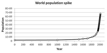
Fig. 1. Spike-like growth of the world population in the last two millennia (data from Maddison [Devezas 2009; Maddison 2007b])

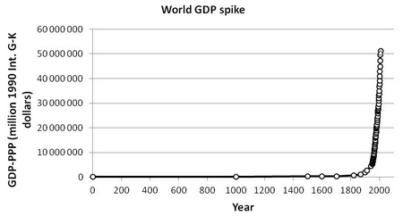
Fig. 2. Spike-like growth of the GDP in the last two millennia (data from Maddison [Devezas 2009; Maddison 2007b])

On the other hand, one can ask: Is that really so? Is there a real menace pointing to a possible worldwide catastrophe that could definitively jeopardize human life on Earth? Another question then naturally emerges: could not Gaia as a resilient system find its own way out of this apparently imminent disaster? As will be seen in our analysis ahead in this paper, this kind of graphs evincing explosive growths is always misleading and used frequently for apocalyptic propaganda. In order to get the correct conclusions about the real trends we should look for the details hidden behind the considered growth phenomenon and this is usually done expanding the x-axis and narrowing the focus on its unfolding in shorter time spans.

We know that this is a very controversial theme of debates and equally know that there are many scientists voicing against the exaggeration of simple extrapolations of the observed trends. Our objective in this work is not properly to deliver answers about this scientific puzzle, but the fact is that the approach we are pursuing in last years and the results of our ongoing research, as well as the results of other recent investigations, point to this very concrete possibility – the World System is approaching an Era of Transition that will conduce naturally to a new order within which these troubles will be overcome. What we do not know yet is if this transition will be a smooth one or much on the contrary, a very turbulent one as already happened in the past. We hope that the present results may help in shedding some light on the road ahead.

We have already pointed out that Devezas and Modelski(2003) have demonstrated that the World System is prompt to a very important transition and demonstrated that the dominating order has already reached 80 % of its millennial learning path (see Devezas and Modelski 2003: fig. 9). In another recent work Devezas et al.(2008) have shown that the increasing efficiency of energy systems is following an irreversible path toward the usage of carbon free energy sources, a process that will be completed before the end of the present century (see Devezas et. al. 2008: figs 10 and 11).

Very recently econophysicists Johansen and Dornette(2001) have given an important contribution in this direction. They have shown that, contrary to common belief, both the Earth's human population and its economic output have grown faster than exponential (i.e. in a super-Malthusian mode). These growth rates are compatible with a spontaneous singularity occurring at the same critical time around 2050 signaling an abrupt transition to a new regime. But the abruptness of this transition might be smoothed, a fact that can be inferred from the fact that the maximum of population growth was already reached in the 1960s, in other words, a rounding-off of the finite-time singularity probably due to a combination of well-known finite-size effects and friction, suggesting that we have already entered the transition region into a new regime.

Closing this section it is shown in Fig. 3 the spike-like growth of the Dow Jones Industrial Average (DJIA) considered weekly from 1900 until September 2009, and in Fig. 4 the historical growth of gold price for the same time span, also considered weekly. In the case of gold, which will be subject of a detailed analysis ahead in this paper, we do not have what can be coined as a spike-like growth, but anyway it can be observed a spectacular growth with wild oscillations, exhibiting two very strong peaks separated by approximately 30 years.

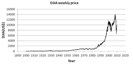
Fig. 3. Dow Jones Industrial Average weekly price since 1900 until September 2009 (Analize Indices... n.d.)

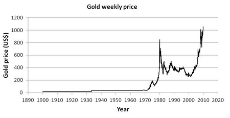
Fig. 4. Gold weekly price per troy ounce since 1900 until September 2009 (Kitco n.d.)

5. Signals of Saturation

Let us begin looking at the evolution of the two most important agents, Earth's population and its aggregate output, but initially narrowing our observation to their recent unfolding after 1950, a period for which the most reliable data are available.

In the previous section we have already pointed out the fact that human population growth rate has already reached its maximum, as depicted in Fig. 5. A peak of 2.2 % was reached in 1962–1963, and after this date has decreased steadily being nowadays of the order of about 1.13 %. Looking another way around, the annual change in the world population peaked in the late 1980s when the world population experienced a net addition of about 88×10⁶ individuals (obviously because the population in the 1980s was much bigger than in the 1960s). These figures were taken from the International Data Base of the U.S. Bureau of Census (n.d.), whose estimate for the world population in 2050 is of about 9.316×10⁹ people.

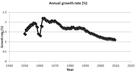
Fig. 5. Annual rate of growth of the world population 1950–2009 (U.S. Bureau of Census.URL: http://www.census.gov/population/international/data/idb/worldgrgraph.php)

An important point to refer about the Fig. 5 is the pronounced dip appearing in 1958–1960 that was due to the so-called Great Leap Forward that occurred in China in this period, amidst with natural disasters, widespread famine and in the wake of a massive social reorganization that resulted in a toll of tens of millions of deaths. As we will observe in the next section, this dip is also very visible in the historical evolution of the world GDP and warns us about the weight of China and its very important role in economics-related world affairs.

Curiously, and in despite of the data (calculations!) of the U.S. Bureau of Census, the recent evolution (since 1950) of the world population can be finely fitted by a logistic curve, which delivers a slightly different result regarding both – the extrapolation to the year 2050 and the turning point corresponding to the maximum growth rate. This fitting is shown in Fig. 6a (the logistic curve) and 6b (the same in the form of a Fisher-Pry plot), which were obtained using the IIASA's LSM II program (IIASA 2011). As can be observed the fitting is absolutely perfect (R² = 1), what implies that we are amidst a natural growth process, with a characteristic time Dt of about 160 years (1920–2080), with an inflexion point in 2000–2001 (maximum growth rate). The maximum carrying capacity of this process points to a population of about 12×10⁶ people to be reached by the end of the century, but that can stabilize before this maximum (say by about 10×10⁹ people, considering that the end of a logistic growth process implies the transition into a new regime). Our curve points to a population in 2050 of about 9.7×10⁹ people.

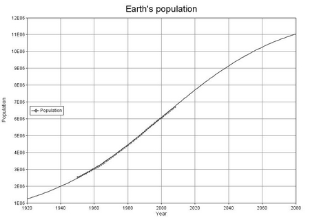
Fig. 6a. Logistic growth of the world population 1950–2009 using IIASA’s LSM2 software(IIASA 2011)

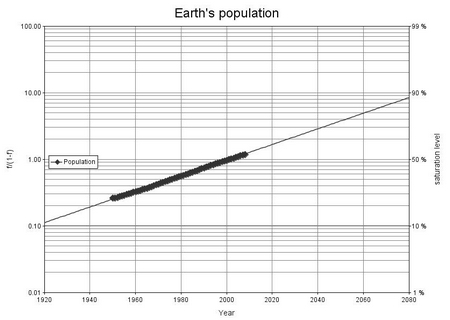
Fig. 6b. Fisher-Pry plot of the world population 1950–2009 using IIASA's LSM2 software (IIASA 2011)

In recent paper Boretos(2009) performed the same fitting using the U.S. Bureau of Census' data set until 2005 and has found a somehow moderate result, with a characteristic time Dt = 117 years and a turning point in 1995. Accordingly to the set of data used by this author the extrapolation to the year 2050 matches the projection of the U.S. Bureau of Census.

Let us now call our second agent, the aggregate world output, or in other words, the world GDP. Using Maddison's data since 1950 we have also fitted a logistic curve and the result is depicted in Fig. 7a (logistic curve) and 7b (Fisher-Pry plot). The fitting is not so perfect (R² = 0.996) as in the previous case of Earth's population, but works equally well.

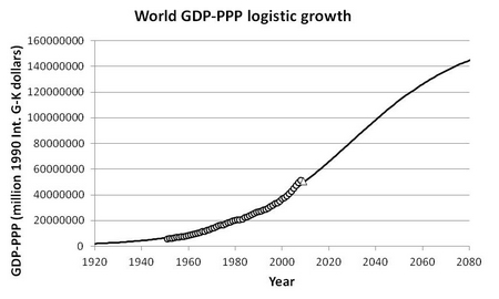
Fig. 7a. Logistic growth of the world GDP-PPP 1950–2008. The last point (triangle) is the estimate for 2009 from IMF (2009)

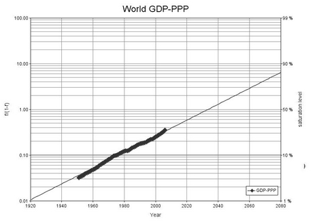
Fig. 7b. Fisher-Pry plot of the world GDP-PPP 1950–2008. The last point (triangle) is the estimate for 2009 from IMF (2009)

The resulting logistic corresponds to a natural growth process with a characteristic time Dt ~ 110 years that will saturate about 2080 with a turning point (peak of the growth rate) around 2030. Boretos(2009) has tried the same fitting using a different dataset and numbers only until 2005 and has found a similar result with a characteristic time of about one century and a turning point in 2015. Unnecessary to stress that these differences are absolutely irrelevant considering that we are using different datasets and in our fittings we have used more recent data (until 2008), which has naturally contributed to a slightly higher carrying capacity and pushed the turning point ahead in time. The main reason for this difference lies in the higher world GDP growth rates observed in the period 2006–2008, which we will further analyze in the next section.

These results require some further thought. What is the meaning of these natural growth processes? Why the GDP has grown faster than population? There are no simple answers to these questions and their deep analysis deviates from the purpose of this piece. But a few words about their meaning are worth putting.

Human population and its output are growing since the onset of civilization some five millennia ago. But contrary to a widespread impression, the story of world population of the last 5000 years is not one of continuous exponential growth. Rather, it can be best described as a series of three major surges, each more substantial than its predecessor, but both of the first two surges also followed by a long period of population stability(Devezas and Modelski 2003). The graph depicted in Fig. 1 shows only the last stable period and the last spike-like surge respectively. As already shown by Devezas and Modelski(Ibid.), this 2000-year process corresponds to the formation of the global system, one of the global-institutional processes that monitor the progress of agents, and program their developments. Nested within this longer process there are other shorter global-institutional processes like the global economy process (~250 years; see Ibid.: table 2) that corresponds to the process being analyzed in this paper.

At this point we wish to make stand out the first important result of the present investigation, which can be easily discerned through the comparison between the actual points and the path of the logistic growth process shown in Figs 7a and 7b. In these graphs we have also included the estimated projection for 2009 (the triangle in both graphs, using data from IMF [2009]). As can be seen the actual points, mainly between 2005–2008, evidence a slight deviation upwards, and the point corresponding the estimate for 2009 seems to pull the curve downwards in order to match the original path. In order words, the present crisis seems to work as a kind of self-correction mechanism of the system.

The next step was to look at the behavior of the unfolding of the global output per capita. Using the recent data the fitting of a logistic curve does not work well, a result that diverges from those got by Boretos. In fig. 4 of his paper this author shows a logistic fit, but the substitution curve is clearly right skewed and the author does not present the error estimates. Boretos (2009) states that world GDP has increased faster than population at all times, but this is not true as alias we can infer from the linear fitting of the GDP/capita exhibited in Fig. 8 below.

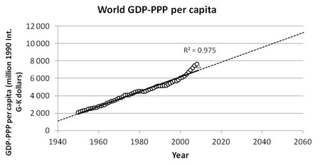
Fig. 8. Linear fitting of the world GDP-PPP per capita 1950–2008. The last point (triangle) is the estimate for 2009 from IMF (2009)

As can be observed the overall linear fitting is not bad (R² = 0,975), but most important the linear trend is perfect until 1981, deviating downwards after this date and until at least 2001, what implies a growth rate of GDP below the population's growth during approximately a time span of 20 years. After 2004 and until 2008 the actual data exhibits an inverted behavior, that is, the world GDP has grown faster than population – but this trend stopped abruptly in 2009. Again the extrapolated point that contains the outcome of the actual crisis seems to pull the trend downwards. It is clear that if we use the extrapolation for 2010 the corresponding point will be located still closer to the straight line.

Resuming the results of this section we have:

1. The present crisis seems to be a kind of self-correction mechanism that brought the global output back to its original logistic growth pattern.

2. This pattern corresponds to a final phase of the ongoing global economy process, which will saturate before the end of this century, signaling that we are entering into a new regime (a new learning process) of the socioeconomic world system.

In the next sections we will see how results from other analysis and approaches reinforce these preliminary conclusions.

6. Comparative Analysis of the Global Output under a Larger Timeframe

Fig. 9 shows the timely evolution of the GDP-PPP for a set of 18 selected countries for which the most complete data are available since 1870. These countries together contribute today for ~70 % of the global GDP (74 % in 1950, and 73 % in 1970). This result is well known; everyone is acquainted with the fact that China is the country exhibiting the most dramatic GDP growth during the last decades, and certainly will surpass the USA in the next decade or so. India and Brazil are also growing at fast paces, but still far below China, while Europe and Japan demonstrate that they are losing momentum in this race. It is very evident that the former USSR was hit at the late 1980s by its political-economical transformation and disaggregation, but is also recovering momentum led by Russia and some of their former members.

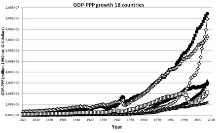
Fig. 9. GDP-PPP growth 1870–2008 for 18 countries – USA (^■), China (à), 12 Western European countries (∆), India (▲), Japan (●), former USSR (^□), Brazil (x)

This kind of graphical representation does not allow to discern details and much less to perform reliable forecasts. On the other hand, the picture is completely different if we look at annual movements in aggregate activity, or in other words, the annual growth rate of GDP. As will be seen in this section, such visualization allows discerning changes that have appeared systematically across countries, due to catastrophes, political and/or social upheavals, wars, recessions, etc. Moreover, it permits also to distinguish some patterns, as for instance the different phases of K-waves observed since 1870.

In figure 10 that follows it is depicted the historical record since 1870 of the annual growth rate of the world GDP-PPP using Maddison's data. Before advancing commenting on some important details of this picture, it is important to clarify some aspects considered in the construction of this graph.

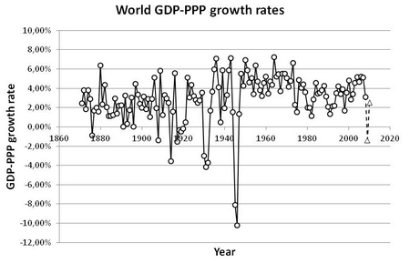
Fig. 10. World GDP-PPP growth rates 1870–2008 (data from Mad-disson 2007b). ∆ – Estimates for 2009 and 2010 from IMF (2009)

As already explained in the third section of this work, Maddison's data set is not complete for the entire time span since 1870. For the construction of the graph shown in Fig. 10 the data corresponding for the interval 1870–1884 are the numbers for USA and 12 WE countries, where undoubtedly at this time the leading economies in the world (in 1880 corresponding to 55 % of the world GDP). Between 1885 and 1927 the numbers include also India, Japan, Indonesia, and Brazil (in 1900 corresponding to ~61 % of the world GDP), and between 1928 and 1949 the USSR was added to this group (corresponding in 1940 to ~71 % of the world GDP). From 1950 onwards the numbers include all countries.

The validity of this approach can be inferred from the behavior of the two superposed graphs shown in Fig. 11, showing the unfolding of the GDP growth rates for the world and for the USA plus 12 WE countries. As can be observed, the movements – ups and downs – are perfectly ‘in phase’, the only clearly observable difference is that the peaks (maximum growth rates) and dips (minimum growth rates) for the world are damped, due to the fact that the performance for some individual countries are not exactly synchronized with the leading countries. This ‘damping effect’ seems to work well until at least the year 2000, when an opposite effect seems to enter in action. But the general aspect of the graphs suggests clearly that the USA plus the 12 WE countries leaded the world economy for the most of the time.

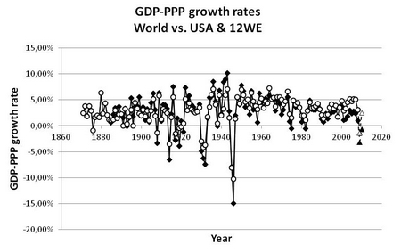
Fig. 11. Comparison between the GDP-PPP growth rates for the world (○) and USA plus 12 WE (♦). The last points ∆ (world) and ▲ (USA + 12 WE) are the estimates for 2009 and 2010 from IMF (2009)

The picture is completely different when we compare the behavior of individual countries, like India and China (data for China are shown only after 1950), both with very troubled history, as shown in Fig. 12 in comparison with the same world graph. It is very clear that the fluctuations are much more radical for the individual countries and not synchronized with the rest of the world.

Note that estimates for 2009 and 2010 (from IMF) were included in all these previous graphs. It is also important to point out that we have not used weighted averages in these graphs; weighted averages contribute to a biased picture of the whole. What we have in all three graphs represent the very fluctuations of the aggregate output.

Fig. 12. Comparison between the GDP-PPP growth rates for the world (○), India (▲), and China (à). The last points world (∆), India (^■) and China (^□) are the estimates for 2009 and 2010 from IMF (2009)

Now let us try to present in a resumed form, point by point, the main aspects unveiled when looking at these graphs, or in other words, when observing the secular unfolding of the aggregate world output.

1. The most striking aspect exhibited by the graph in Fig. 10 is the very turbulent time during the first half of the 20^th century, which carried within with the effect of two world wars and the most painful economic crisis already experienced by the world economy; note that the ‘dip’ corresponding to this Great Depression is placed exactly in the middle of the ‘double dip’ corresponding to the two world wars, roughly equidistant by ~15 years.

2. This turbulent time is confined between two periods of ‘peace times’, the first one from 1870 until 1913 (then 43 years), and the second one from 1950 until 2008 (then 58 years).

3. The first period of relative stability and ‘peace times’ is marked by two pronounced dips with negative growth rates, a first one in 1876 and a second one in 1908. The first dip corresponds to the panic of 1873, which gave place to a strong recession of the world economy, but that was especially severe in the USA. The NBER[1] statistics (NBER n.d.) consider it as the longest recorded contraction cycle in the USA (65 months, 1873–1879), and some authors(Nelson 2008) have compared it with the current financial crisis due to many common characteristics. The second dip appears in 1908 and was a consequence of the panic of 1907(Bruner and Carr 2007), with also dramatic global consequences, but shorter in duration (in the NBER statistics [Ibid.] for the USA a contraction cycle of only 13 months). Despite its short duration it can be considered as a Great Recession comparable in numbers (GDP contraction) to the present crisis.

4. Still regarding this first ‘peace times’ period, we can distinguish two subperiods: one with a downward trend (decreasing growth rates, considering the mean values) that extended until at least 1896, soon followed by one with an upward trend (increasing growth rates, considering the mean values), that extended until the middle 1920s but was disturbed by the onset of the WWI. We have then two subperiods: ~1870 to 1896 and 1896 to 1922, each with ~26 years, that as suggested by many adepts of Kondratieff long waves correspond respectively to the downwave phase (or phase B) of the 2^nd K-wave and to the upwave (or phase A) of the 3^d K-wave.

5. Regarding the second ‘peace times’ period that followed WWII and started after 1948, we can more easily distinguish different subperiods – more exactly three. A first one located between 1948 and 1973, when the global output averaged a growth rate of about 5 %, a second one between 1974 and 1992, when the global output averaged circa 3.5 %, and a third one after 1993 when an upward trend is observable, reaching and surpassing the mark of 4 % (with a brief interruption in 2001 – the dot.com bubble). The reader should note that there is a dip in the world-series corresponding to 1998, but comparing with the graphs shown in Figs 11 and 12 we can see that it was not a crisis in the USA or Europe, but the consequence of the famous Asia Crisis (Kaufman et al. 1999), which started in July 1997 in Thailand and spread quickly to many other Asian countries, including China and India. Again we have subperiods with time spans averaging two decades – in this case now 25 years and 18 years respectively. K-waves' adopters usually associate these subperiods with the up and downwave phases of the 4^th K-wave. Following this schema it seems that after 1992 the 5^th K-wave might already be started. We will turn to this point in the next section.

6. Regarding now the actual crisis, translated by the extrapolated points for 2009 and 2010 (small triangles in Fig. 10), we cannot draw so easily the same conclusion expressed in the previous section of a self-correction mechanism that is pulling the general trend towards its original path. The points for 2009 and 2010 resemble much more a pathological symptom signaling that something is wrong with the existing economic system, or perhaps more exactly expressed, with the existing global financial system. We use here ‘a pathological symptom’ because we are facing neither a world war, nor a worldwide social upheaval. Something else seems to be hidden behind the facts.

7. A closer look again to our graphs of Figs 10, 11 and 12 may help to shed some light upon the facts. A very important detail to stress is that we have historically a very important precedent that happened in 1907, that is, exactly one century ago (or, in other words, two K-waves ago!). The phenomenon, known as the ‘1907 Bankers Panic’ (Bruner and Carr 2007), was very similar to the actual crisis under at least two important aspects: it occurred during an upward trend of the global economy (i.e. during the A-phase of a K-wave) and was a pure financial crisis involving market liquidity that led to bankruptcy of many important agents of the banking system, which quickly spread from New York to Europe and to some Asian countries (see for comparison graph of Fig. 12). The remedy at that time was the same as nowadays: the injection of large sums of money to shore up the banking system, soon followed by a profound reform of the U.S. financial system, which included the creation of the Federal Reserve System (FED, created in 1913). The reader should observe in the graph of Figs 10 and 11 that the dip in 2009 mirrors the one in 1908!

8. As already referred to in the paragraph preceding Fig. 11, it is very evident from the graphs comparing the unfolding of the world GDP and the sum of the USA plus 12 WE GDPs, that after 2000 a different trend emerged: the growth rates of the world GDP from this date onwards are higher than for the USA and the European countries together, an inverse behavior of the GDP evolution to this date. This push upwards is clearly motivated by the rocketing GDP growth rates observed for India and China, as can be inferred from Fig. 12.

9. Such an inverted trend seems to be a clear signal that we are already witnessing a transition to a new global socioeconomic system, which will carry with a profound restructuration of world economic affairs. In a few words it means that real growth rates of low-income countries have been growing increasingly apart from those of high-income countries. See more details in the Conclusions.

10. Ajar with the times, the present crisis seems to sum up a mix of self-correction mechanism (or at least the urgent necessity of finding the necessary measures for correction) and signals of an imminent transition to a new world order.

Before closing this section it is worth bringing to the reader's attention the fact that negative fluctuations of the world GDP are not sufficient condition to characterize a great depression. There are more things at stake when we wish to speak of economic recessions with a worldwide impact and severe consequences across countries. In a very recent book the economists Carmen Reinhart and Kenneth Rogoff(2009) have shown that in order to characterize a real great depression it is necessary to observe not only a considerable contraction of the GDP, but also a significant retraction of the worldwide commercial exchange. For these authors this phenomenon has only occurred three times in the recorded history: in 1907/1908, 1929/1933 and now in 2007/2009. Many other crises, like those of 1873/1879, 1945/1946, 1987, 1998 or 2000/2001, have not had the same global impact like these three mentioned, because they have not hit equally both measures (GDP and commerce) or have had only regional effects (like the 1998 Asian crisis). This aspect is a very important one regarding our previous conclusions and the parallel between the actual crisis and the 1907 Panic.

7. Scrutinizing the Recent Record of the Global Output

Keeping in mind the fact already mentioned in our fifth section (Signals of Saturation) that the most reliable data for the global output are those that followed WWII, it is worth scrutinizing further this recent period, which we coined as the second ‘peace times’ period.

Fig. 13a shows the result of applying an 11-year moving average to the data of Fig. 10 (world GDP-PPP growth rates) in the period 1947–2008. As can be seen it is evident a wave-like behavior suggesting the fingerprint of a complete long wave. Fig. 13b presents the result of fitting a simple sinus series of the type P(t) = P₀ + A sin (2p t/T) + B sin² (2p t/T) + …, whose solution is P(t) = 4 + 1.03 sin (2p t/50.14) + 0.03 sin² (2p t/50.14), evincing then a periodical movement with a period of about 50 years (the points for 2009 and 2010 were not included in the fitting).

This result comes to reinforce our conclusion resumed in point 5 of the previous section that we can divide this recent period in three subperiods – the first and second corresponding to an entire K-wave and the third corresponding to the upward movement of the following K-wave. The entire K-wave in this curve matches very well the dates that many different authors have presented for the 4^th K-wave, which started about 1947/48, reached a maximum about the 1970s, and was completed in the first half of the 1990s.

The extrapolation for the fifth K-wave points to a maximum to be reached shortly before 2020, or in other words, the present expansion movement, although disturbed by the recent crisis, may well continue for more one decade. The much discussed apparent recovery still on course (crisis 2007/2009) seems to hint that the system is indeed resilient.

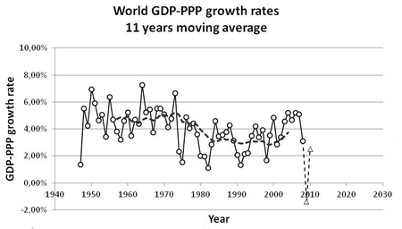
Fig. 13a. 11-year moving average applied to the world GDP-PPP growth rates in the period 1947–2008. The estimates for 2009 and 2010 (∆) were not included in the MA

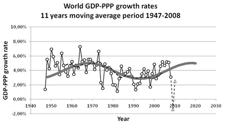
Fig. 13b. Result of fitting a simple sinus series P(t) = 4 + 1.03 sin (2p t/50.14) + 0.03 sin² (2p t/50.14), evincing a periodical movement with a period of about 50 years (the points for 2009 and 2010 were not included in the fitting)

8. Shrinking Recessions and Contractions

In a recent paper the Italian economist Mario Coccia(2010) brings to attention the fact that the duration of business cycles' contraction phases are far shorter than the duration of expansion phases. The author observes also that the duration of the recessions corresponding to the downwave phase of a long wave is in average shorter than the upwave phase. In the case of business cycles the author uses statistics from NBER (n.d.) and from the U.S. Bureau of Economic Analysis (BEA),[2] comparing data for the USA, the UK and Italy. In the case of long waves the author uses an extensive comparison of the dates proposed to this phenomenon by many different long-wave theorists.

His results point to a mean duration of business cycles' contractions in the USA, between 1854 and 2001, of about 17 months, and a mean duration of expansions of about 39 months, or in other words, an average of 31 % of the time experiencing economic contraction and 69 % experiencing economic expansion. Regarding the K-waves the author points to an average of about 29 years for upwaves (53 % of the total time) and 26 years for downwaves (47 % of total).

In this research we decided to explore also this phenomenon using the NBER statistics for the USA and were confronted with two very interesting and unexpected results: first, there exists an increasing trend towards shorter contractions and longer expansions, and second, the fingerprint of K-waves is clearly visible also in the history of the U.S. Business Cycles.

Fig. 14a shows the graph resulting from the distribution in time of the succession of economic expansions and contractions in the history of business cycles in the USA since 1850. In despite of the star field-like aspect of the distribution of the points, one can clearly distinguish the enduring trend towards longer expansions and shorter contractions translated by the straight trend line. The last point in this graph corresponds to the expansion period that lasted from the end of 2001 to the end of 2007 (73 months) and ended with the onset of the actual crisis.

Fig. 14b presents the resulting 20-year moving average applied to the same historical statistics. The trend line reveals a wave-like behavior that coincides with the dating schema used by many long-wave authors and matches very well our conclusions in the previous sections. In this graph we have added a point to the actual crisis considering it with a supposed duration of 24 months. This point was considered in the moving average in order to observe the path of the trend line. Again we are induced to the same conclusion drawn in point 1 at the end of the fifth section (Signals of Saturation) – this last point suggests the action of a self-correction mechanism bringing down a period of excessive growth!

Coccia(2010) suggests that these shrinking contraction periods may be due to a learning process during which government(s) have developed functioning methods to undermine the effects of economic recessions. This suggestion comes to reinforce our second conclusion in the fifth section about a secular learning process of the socioeconomic world system.

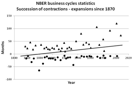
Fig. 14a. Star field-like aspect of the distribution of the succession of economic expansions (▲) and contractions (●) in the history of business cycles in the USA since 1870 (NBER n.d.). The straight trend line translates the trend towards longer expansions and shorter contractions in business cycles

Fig. 14b. 20-year moving average applied to the points of Fig. 14a. The trend line reveals a wave-like behavior that coincides with the dating schema used by many long-wave authors corresponding to the 2^nd, 3^rd, 4^th and 5^th K-waves. In this graph we have added a point (○) corresponding to the actual crisis considering it with a supposed duration of 24 months

9. Maddison's Phases of Economic Growth

In a publication from 2007 Maddison(2007a) performs a balance of his impressive and massive historical research about the evolution of the world GDP and GDP/capita since the beginning of the 19^th century, as well as a detailed analysis of the works of some long-waves theorists (Kondratieff, Kuznets, Abramovitz, Schumpeter, and long-wave revivalists like Rostow, Mandel and Mensch). Maddison concludes that the existence of a regular long-term rhythm in economic activity is not proven and states further that there is no convincing evidence to support the notion of regular or systematic long waves in economic life.

Based mainly on his own data on aggregate performance Maddison however concedes that there have been major changes in growth momentum of capitalist development since 1820, which he coins as phases of economic growth. He recognizes five phases: 1820–1870 (transition from merchant capitalism to industrial accelerated growth), 1870–1913 (liberal phase), 1913–1950 (beggar-your-neighbor phase), 1950–1973 (golden age), and a last one from 1973 onwards (neo-liberal phase). Curiously there is some coincidence between these dates and some very important dates used by long-wave adopters either to characterize the duration of a full wave or to mark the transition between phases (up and down) of long waves.

But there are some oddities to point out in Maddison's whole analysis. In first place his review of authors contributing to bring empirical evidence on the existence of long waves is far from complete and does not include very important vast research work of authors that have brought robust empirical evidence using most effective mathematical tools. Maddison reviews basically only classical authors that have tried either to advance economic models to explain the long-wave phenomenon or to present evidence based only on economic statistics (with the exception of Mensch).

As robust empirical and mathematical evidence one must considers at least two authors that have carried during decades (1980s and 1990s) extensive work on long waves: the American economist Brian Berry and the Italian physicist Cesare Marchetti, whose works were published in the pages of TF&SC and elsewhere. Berry(1991) used convincingly chaos theory and spectral analysis to prove the existence of long waves and Marchetti,[3] leading a research team at the International Institute for Applied Systems Analysis (IIASA), produced some hundred graphical analyses applying the logistic substitution model on physical measures of human aggregate activities. In our point of view there is a touch of nonsense and exaggeration in simply refusing all the massive evidence brought by both authors.

Indeed it is very difficult to prove the existence of long waves using only economic statistics. There are many variables that must be considered simultaneously and this consists in an almost impossible task. But we must recognize that in despite of this inherent difficulty there is the register of at least two bold forecasts in recorded history: Kondratieff himself, writing between 1922 and 1926, predicted accurately the Great Depression of the 1930s and there is the famous graph published in 1974 by Media General Financial Services that had been widely reproduced by dozens publications on long waves since then (the graph was also reproduced in one of our previous publications in the pages of TF&SC[Devezas and Corredine 2001]). This graph, a schematic depiction portraying the cresting unfolding of K-waves since the 1790s, predicted also very accurately the behavior of the world economy in the following decade (the 1980s), when was observed a global reduction of economic growth and retraction of the world commerce, as alias evinced too through the timely evolution of the world GDP-PPP growth rates shown in Figs 13a and 13b.

This kind of schematic depiction of K-waves has been the preferred target of many criticizers of Kondratieff waves, who insist on the fact that such regular long-term oscillations do not exist. It is clear that such a monotonic upward movement during about two decades, followed by a subsequent two decades-long downward movement does not exist indeed – what is necessary to comprehend is that such a representation is just a schematic portrait of very complex behavior that includes the timely unfolding of several variables and does not try to translate the evolution of a unique variable. Perhaps, a bit more realistic representation should include in the upward and downward movements the within nested shorter business cycles, as we try to express through Fig. 15. But again it is very important to stress that this is just a schematic depiction of a much complex phenomenon and does not intend under no circumstances to render a real depiction.

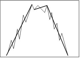
Fig. 15. Schematic depiction of a hypothetic long wave with nested shorter business cycles. As explained in the text this is just a schematic portrait of a very complex phenomenon and does not intend to render a real depiction of a single variable

As a second oddity in Maddison's whole analysis we wish to point out the lack of graphical analysis. One really wonders why Maddison does not use graphs in his publications. In his famous and very frequently referred book(Maddison 2007b), for instance, among 124 tables, Maddison presents only seven graphs, and just for comparisons of GDP cumulated growth (or comparative levels of GDP/capita) for pairs of countries, like UK/Japan, UK/India, US/China, etc. In his own wordshe says to use ‘inductive analysis and iterative inspection of empirically measured characteristics’ (Idem 2007a: 147), but the most of his analysis and conclusions are drawn only based on tabular constructions, which do not allow perceiving long-term trends and details of an evolutionary process. As can be seen in this work, a simple glance at some graphs allows the perception of fingerprints of K-waves, as well as the observation of details related to the temporal behavior of a given economic-related quantity.

It is hard to understand why Maddison is so adamant in his statements about the lack of evidence on K-waves if he has never applied mathematical analysis on his monumental set of data, as for instance spectral analysis. We have already mentioned above the contribution of Brian Berry. This author, in his 2001 paper(Berry et. al. 2001) has demonstrated the existence of low frequency waves of inflation and economic growth using digital spectra analysis. He and his collaborators have found ~9 and ~18-year oscillations linked to business and building cycles, and additional ~28 and 56-year rhythms linked to inflation alone.

Very recently Korotayev and Tsirel(2010) have examined minutely the entire data set of Maddison's GDP-PPP growth rates under the optic of modern spectral analysis and have found very similar results, or in other words, two strong frequency peaks corresponding to the shorter business cycles (in this case ~8 years and ~15 years), and two long-term frequency peaks (~30 and ~52 years) related to long waves – the shorter probably corresponding to upwaves and downwaves movements and the longer corresponding probably to complete K-waves oscillations.

In our research we decided then to verify these results and have applied a simple Fast Fourier Transform using the Sigview software.[4] The result is shown in Fig. 16 where we can clearly discern the existence of four frequency peaks, in this case 7.5 years, 15 years, 32 years (very weak) and 52 years – again practically the same result as those of Berry and Korotayev-Tsirel. It is important to stress that ours and Korotayev-Tsirels' results were found in the same data set where Maddison says that there is no convincing evidence to support the existence of systematic long waves in economic life.

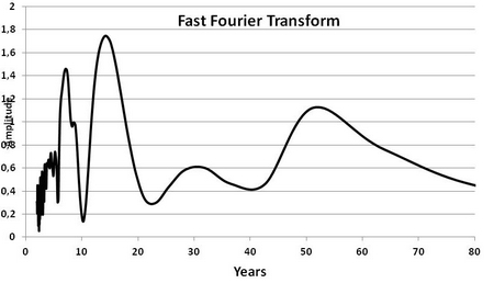
Fig. 16. Fast Fourier Transform using the Sigview software(Kondratieff 2004) applied to the historical unfolding of the GDP-PPP growth rates presented in Fig. 10. We can clearly discern the existence of four frequency peaks: 7.5 years, 15 years, 32 years, and 52 years

Closing this section we wish to briefly discuss a statement of Maddison, where he wrote:

The government regulatory role in the economy has greatly increased. One result of the latter is that the stability of financial institutions has improved. Before the Second World War, depressions were often reinforced by major bank failures, but these are now rarer and their impact is cushioned (Maddison 2007a: 161).

What is curious in this statement is that it is partially true – in fact, there have been a learning process during which governments have learned a lot how to reduce the impact of economic shocks, as we have already stressed previously, and that explains the phenomenon of shrinking recessions and contractions portrayed in the Fig. 14a. But on the other hand, it is completely false regarding the stability of financial institutions. Let us give a discount to Maddison – he has written these lines shortly before the big financial crash of the end of 2007.

10. Gold – the Master of Commodities

At the end of the closing chapter of his 1922 book Kondratieff (2004) has made a very important observation about the behavior of gold during the unfolding of K-waves, which has been bypassed by most of long-waves analysts up to present days. In this chapter, with the suggestive title ‘The crisis of 1920–1921 in the system of general movement of conjunctures’ Kondratieff paved the way for his dangerous idea of an incoming (temporary) collapse of the world economy and used gold to reinforce his damned prophecy. The inclusion of the word ‘temporary’ here is very important, because Kondratieff's dangerous idea was not the forecast of a final collapse (as wished by his Bolshevik opponents), but the anticipation of a new downward wave, which should be followed by another upward wave – or, in other words, a general picture of a wave-like movement of the capitalist system.

Kondratieff wrote:

Gold output, on the other hand, showed a remarkable movement, too. Since mid-1890s its output was surging to come to a maximum in 1915 and a subsequent continuous decline… The output of gold is quite likely to plunge into a long depression, which is the most remarkable feature of the current epoch (Kondratieff 2004: 121).

He follows referring to a study of Joseph Kitchin and presents a table from a publication of this author with data about the annual average growth of gold output, in which can be seen a minimum in 1810, a maximum in 1847, again a minimum in 1868, followed by a new maximum in 1891, and declining again after this date. In the following paragraphs he wrote:

It can be readily seen that the dates and periods displayed match closely the turnarounds and periods of upward and downward waves of the long cycles. It is also quite obvious that the upward waves are coincident with periods of a high annual growth of gold, and vice versa. In this case, we enter upon the area of relatively low annual growth of gold, which is going to affect the downward conjunctures of the long cycle… Again this process promises to follow the line of the 1870 (Kondratieff 2004: 141).

Indeed a bold forecast and what happened in the following years is the history everyone knows very well. But after these lines Kondratieff has made also another very important point:

We can therefore relate to the world economy as being quite likely to enter upon a downward phase of the long cycle. This by no means goes to say that this phase will be clear of its own ups or downs or depressions in terms of minor capitalist cycles. They have always been present in such phases in whatever long cycles of conjunctures of the past. They will surely be present in a downward phase of the long cycle. In a general frame of their variation, however, the conjunctures are most likely to keep downwards. Consequently, elevations in minor cycles of the oncoming period will lack the intensity they would display while on an upward wave of a long cycle. By contrast, crises of this period promise to be sharper, and depressions of minor cycles lengthier (Kondratieff 2004 [1922]: 142).

Again a bold forecast, and the reader must keep in mind that these lines were written in 1922. What Kondratieff voiced in this last paragraph is exactly what we have tried to express through Fig. 15 in Section 8.

The question now is: What does our important actor in world economic affairs, gold, allow us to say about the present trend and what may be forecasted regarding the forthcoming years? As we will see some forecast is indeed possible, but we have first to consider that the behavior of gold has changed dramatically along with the last century, after Kondratieff inspired vision.

The graph depicted in Fig. 4 (Gold weekly price) cannot tell us much about the future of gold price, except perhaps the fact that we are presently witnessing a strong momentum upwards. Such growth however cannot continue indefinitely, nothing in the universe growths forever. But on the other hand, this graph tells us a lot about the gold's past and recent history. As can be seen, since 1900 gold experienced a long period subjected to two levels of constant prices until 1971, when suddenly began to raise, reaching a first modest peak in 1975, soon followed by a strong peak by the end of 1980, outreaching the level of US$ 800. This record was immediately followed by a continuous trend of decreasing prices that endured for 20 years, reaching a minimum of about US$ 270 by the end of 2000, when gold entered a new phase of an apparently unstoppable trend towards ever increasing prices.

The long period of constant prices belongs to the old times of the ‘gold standard’, which started in Britain after the Napoleonic wars. In the second half of the 19^th century, a number of nations in Europe and elsewhere followed suit, and the United States adopted the gold standard de facto in 1879, by making the ‘greenbacks’ that the Government had issued during the Civil War period convertible into gold; it then formally adopted the gold standard by legislation in 1900, when our graph begins. By 1914, the gold standard had been accepted by a large number of countries, although it was certainly not universal.

During the 1880–1914 period, the ‘mint parity’ between the U.S. dollar and sterling was approximately $4.87, based on a U.S. official gold price of US$ 20.67 per troy ounce (31.1035 gr) and a U.K. official gold price of £4.24 per troy ounce. This system worked well during almost forty years when the world economy entered the turbulent phase already referred to when commenting on the graph of Fig. 10.

We can state that this first period of relative peace corresponded to the real entrenching stage of a successful international capitalist system, when there were no changes in the exchange rates of the United States, UK, Germany, and France (though the same did not hold for a number of other countries). There were few barriers to gold shipments and few capital controls in the major countries. Capital flows generally seem to have played a stabilizing, rather than destabilizing, role. After the outbreak of the First World War, one combatant country after another suspended gold convertibility, and floating exchange rates prevailed. The United States, which entered the war late, maintained gold convertibility, but the dollar effectively floated against the other currencies, which were no longer convertible into dollars. After the war, and in the early and mid-twenties, many exchange rates fluctuated sharply. Most currencies experienced substantial devaluations against the dollar; the U.S. currency had greatly improved its competitive strength over European currencies during the war, in line with the strengthening of the relative position of the U.S. economy.

But in the very beginning of the turbulent phase that followed WWI (and when Kondratieff issued his first publications!), there was a widespread desire in Europe, especially in the UK, to return to the stability of the gold standard, and a worry about the growing attractiveness of the dollar – which was convertible into gold – and of dollar-denominated assets. Following a disastrous five years back on the gold standard, the UK abandoned it in 1931, and others followed over the next few years.

Things began to worse and after the onset of the Great Depression in 1929 Keynesian economics was the evident remedy found to recover the agonizing patient. In April 1933, U.S. President Franklin Roosevelt through the Gold Reserve Act imposed a ban on U.S. citizens' buying, selling, or owning gold. While the U.S. Government continued to sell gold to foreign central banks and government institutions, the ban prevented hoarders from profiting after Congress devalued the dollar (in terms of gold) in January 1934. This action raised the official price of gold by more than 65 percent (from $20.67 to $35 per troy ounce) and this fact is translated by the first jump to a new level observed in our graph of Fig. 4.

In 1971, when the Bretton Woods system broke down, President Richard Nixon ended U.S. dollar convertibility to gold and the central role of gold in world currency systems ended, giving birth to a new era of complete liberalization of capital flows. The consequences are very clear in the graph of Fig. 4: the dollar and gold floated and in January 1980 the gold price hit a record of US$ 850 per ounce, soon followed by a decrease that endured for almost 20 years. Only after 2000 gold started to escalate reaching new levels again that make look overt the 1980's record. What can be learned from this picture?

The first quite obvious lesson is that the remedy found to fight the system's illness does not hold for a long time. It is as if the doctors (economists) were combating only the symptoms and not really fighting the true intrinsic system's sickness. The relief measures insistently applied until now by mainstream economics consists in failed contra-cyclical policies that systematically overlook some strong forces underlying the global economy. These strong forces are mainly the inexorable human propensity to hoard and the physical-biological imperatives acting upon the complex socioeconomic system. The latter was already analyzed in deep in some of our previous publications(Devezas and Corredine 2001, 2002) and we do not intend to discuss in this paper. It is looking at the former that we can discern some important hints that can help us to correctly read the historical unfolding of the role played by this important actor – gold – in the whole piece of economic capitalist development.

The reason for our title – the master of commodities – lies in the fact that gold is the most hoardable commodity. Gold does not tarnish or fade; it resists the entropic laws of decay, and its high specific gravity contributes to the fact that the opportunity cost of hoarding gold is far lower than that of hoarding any other commodity. Gold is essentially money of last resort and has been the most effective hedge against turbulent times, be they caused by wars or economic depressions. For all over the recorded history humans have shown an inexorable trend to hoard gold bullions and all the sudden changes observed in the unfolding of the graph depicted in Fig. 4 were due to governments measures trying to oppose this strong economic force. Unnecessary to point out that such measures have never worked (in the long range) in favor of the health of the socioeconomic realm. The increasing price trend evinced since 2001 is the clearest proof of the action of hoarding per se.

But in order to draw effective conclusions about the future path of the world economic system is necessary to look at gold's history other way around. In 1977 Berkeley's Professor Roy Jastram in his seminal work The Golden Constant – The English and American Experience, 1560–1976 (Jastram 1977) demonstrated, for the first time, how gold's purchasing power had been maintained over the centuries. Dividing the gold price index by the wholesale price index he found that the Purchasing Power of Gold (PPG) has fluctuated around a broadly mean value. However, Jastram's research ended in 1976, and therefore he barely foresaw the impact of the new era of floating gold price, still at its genesis.

Very recently Jastram's original work was updated by Leyland(Jastram and Leyland 2009) in a research supported by the World Gold Council. The new edition contains two additional chapters (and the relevant statistics) examining the period from 1971 to 2007. The conclusions about the behavior of the Purchasing Power of Gold differ somewhat between the periods before 1971, when the gold price was controlled, and after, when it was free. Nevertheless, one conclusion remains unchanged – that gold maintains its purchasing power over long periods of time even though, over shorter periods, it has fluctuated significantly. But more importantly, this new research demonstrates that now gold moves just the opposite of what it used to do. Before 1971 gold lost value during inflationary spirals, while it appreciated in value during major deflations. The reason was obvious: gold was fixed in price. But after 1971, when the gold was delinked and set free to fluctuate, the price of gold goes up when inflation goes up, and falls when deflation hits.

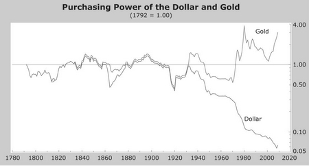
Fig. 17. Purchasing Power of Gold (PPG) compared to the Purchasing Power of US Dollar (PPD) since the 1790s (the American … 2009; Hewitt and Petrov 2009)

In Fig. 17 we present a graph portraying the Purchasing Power of Gold (PPG) and as comparison the Purchasing Power of US Dollar (PPD) since the 1790s recently published in the Web by the American Institute for Economic Research. There are some very important points to infer from this graph that we try to resume below:

1. Both purchasing powers have unfolded perfectly in phase until at least the early 1930s, when they began to diverge and this diversion aggravated substantially after 1971.

2. There is evidently a wave-like behavior and the maxima and minima of the fluctuations before the early 1920s match closely the dates for the turnarounds of long waves pointed out by Kondratieff that we referred to at the beginning of this section; the dip in the early twenties also matches Kondratieff's forecast.

3. The 50-year beat of the maxima of these long fluctuations is absolutely evident – 1840s, 1890s, and late 1930s. Even the peak reached in 1981 falls within the long wave timeframe. It is indeed hard to understand the intestine refuse by mainstream economics in believing in the existence of long waves.

4. In 1971 for the first time in history PPG jumped suddenly from a value below to a value above its historical average, and no more returned to the field below < 1.00. After a brief hesitation in the mid-1970s, PPG rocketed again in 1980–81, when gold price reached the first maximum shown in Fig. 4. This was a decade (1970–1980) not just of high inflation but it also included the two oil price ‘shocks’ and what appeared at the time to be the end of the post-war ‘miracle’ growth of the 1950s and 1960s.

5. After the maximum reached in 1980–1981 PPG entered a 20-year long declining period, during which a self-correction mechanism seemed to act in order to bring it down to its original path along with its historical average. That was the time of the ‘great moderation’ of the decades 1980s and 1990s, a period of disinflation, generally improving economic circumstances, mostly strong stock markets and marked politically by the fall of communism.

6. In contrast, since 2001 the PPG has risen again due to the well-known concern over global imbalances and rising debt, which culminated in the current economic and financial crisis.

7. Comparing the last decreasing period of PPG (1980–2001 = 21 years) with the preceding ones (1842–1870 = 28 years, 1895–1920 = 25 years, 1940–1971 = 31 years) we can say that it was relatively shorter, but not very far away. Associating this fact with the observation that PPG is presently going away from its historical average we can suspect that we are facing an anomaly, or at least we are experiencing a transition phase as we have already pointed out when analyzing other economic indicators.

8. Such an anomaly, or if we prefer, the imminence of a transition phase, is evident from the ‘bifurcation’ (perhaps better, divergence) presented in the graph of Fig. 17. It is quite possible (in fact it is the case since 1971) that a portion of the increase of PPG is really just the outcome of the decrease of PPD, considering that the change in gold price is simply a mathematical recalculation of an ever-changing US Dollar value.

9. The history of fiat currencies is that they lose their purchasing power over time. Because a limited amount of gold exists in the world and paper money can be created without limits, gold has been an ultimate protection against the debasement of currencies. If we look at the historical charts of the purchasing power of major currencies as well as the amount of these currencies in circulation (see, e.g., the graphs presented by Financial Sense University[Hewitt and Petrov 2009]) what we see is that all major currencies have lost steadily purchasing power since 1971 – US Dollar is now at 20 % of its level in 1971, GB Pound at 18 %, Canadian Dollar at 18 %, Australian Dollar at 10 %, Japanese Yen at 70 % and Swiss Franc at 70 %. Opposed to this decrease the amount of circulating paper money of the same currencies grew by a factor 8 (USD), 5 (GBP), 10 (CAD), 20 (AUD), 10 (JPY), and 3 (CHF) respectively. On the other hand, the amount of mined gold has grown slowly and almost linearly, from about 95×10³ metric tonnes in 1971 to about 160×10³ metric tonnes in 2008 (a factor of only 1.6 in more than three decades; [Hewitt and Petrov 2009]). Resuming this point, the amount of available gold (or gold output) is not the cause of the movements of PPG after 1971; the subjacent cause lies in the combination of two other linked factors – an ever-increasing debasement of currencies and declining (1971–1981) or improving (1981–2001) economic circumstances.

10. But supposing that in despite of the changed circumstances the system is resilient and that the PPG will not deviate very much from its historical average (considering also that hoarding has its natural limits), we might conjecture that the actual increasing trend of PPG (and naturally also of gold price) can continue until 2010–2011 (a decade after 2001), but will return to its historical mean value, a process that may involve one or two decades of economic growth that will coincide with the upward phase of the 5^th K-wave peaking about 2020. This forecast matches well our previous considerations when discussing the world GDP.

There is also another way to look at the historical unfolding of gold price calling to playing other of our important agents – the Dow Jones Industrial Average (DJIA). We can calculate a ratio dividing the DJIA weekly index by the weekly price of gold, or in other words, to determine the historical record of the answer to the question: how many ounces of gold does the Dow Jones Industrial index buy? The Canadian financial analyst Ian Gordon originally developed this method, which he uses as an economic forecasting tool. The resulting graph is shown in Fig. 18, and as we can see there is also a clear regular wave-like pattern.

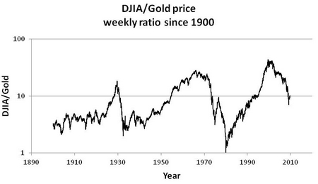
Fig. 18. Ratio DJIA/Gold price considered weekly since 1900. The data used are the same as in Figs 3 and 4

The pattern, however, is quite different from that presented in Fig. 17 – it seems inverted with relation to PPG, some of the PPG peaks are now pronounced dips and the waves have now a skewed aspect, evidencing two or three decades of growth followed by sudden falls. The first quick movement downward was soon after the stock market crash of 1929, and lasted only until 1933, recovering after Roosevelt's Gold Reserve Act. It followed an upward movement during almost three decades, which stopped around 1965–1966 in consequence of a hesitating stock market. In 1971 again a sudden drop after the end of the US dollar convertibility, which extended until 1974 and was followed by the profound dip in 1981 that was due to the combination of a bearish stock market and an accentuated gold rally in prices.

The last wave begins then in 1981 and one can read in this curve the timid stock market crash of 1987, which was followed by a rapid increase of the ratio DJIA/Gold (mainly after 1992), not only due to a worldwide bullish stock market, but also due to the healthy economic growth (and consequently to the cheaper gold) of the 1990s, which the Nobelist Joseph Stiglitz(2003) coined as ‘The Roaring Nineties’. A peak in the ratio happened in 2000, and after the dot-com bubble burst it has followed a steadily downward trend.

The actual situation is one of a hesitating stock market, mainly due to fears of an imminent inflation, and of a gold rally that many financial analysts(Wiegand 2009) want to believe that will continue for a while with gold prices escalating until over US$ 2900! May be such a so high price level will never be reached, but a simple extrapolation of our curve of Fig. 18 induce us to hope that a minimum of the ratio might be reached very soon, which may be soon followed by an upward movement, implying in a recovering economy. Considering also the regular beat of the peaks – 1929–1965–2000, or in other words, a period of about 30–35 years (or a half K-wave), we can speculate that the next peak might be reached by about 2030 or earlier.

Concluding this section we can state that the historical evolution of gold allow us to foresee that the present circumstances of a weakening dollar, a bearish stock-market, and increasing gold prices will reach the end very soon and a renewed economic upsurge may well take place lasting at least until the decade 2020–2030.

Conclusions

In this paper we have investigated the global secular evolution of four important economic-related actors, whose interplay when scrutinized with the suitable analytical tools evince some historical patterns that shed some light on what is going on with the world economic system. These actors are: the world population, the world aggregate output known as Gross Domestic Product (GDP), the historical leader of all commodities – Gold, and the still most important financial index, the DJIA (Dow Jones Industrial Average). Also the succession of economic depressions and expansion periods in the US was examined.

The main conclusions of this research are resumed below:

1. Fingerprints of Kondratieff long waves are ubiquitous in all observed time-series used in this research – world GDP growth rates, succession of economic expansions-contractions in the USA, purchasing power of gold and the historical ratio DJIA/gold price.

2. Regarding the present crisis we can state that it has some unique characteristics, which distinguish it from all previous economic depressions. But in despite of its unique characteristics a parallel with the panic of 1907 may be drawn – both have occurred amidst a strong international growth period and are perfectly symmetric in the observed space-time pattern.

3. The most important conclusion concerning this crisis is that it seems to sum up a mix of a self-correction mechanism that brought the global output back to its original logistic growth pattern, and signals an imminent transition to a new world economic order.

4. The next decade will be probably one of worldwide economic growth, corresponding to the second half of the expansion phase of the fifth K-wave, but that will saturate soon after the 2020s.

5. There are strong signals that we are already witnessing a transition to a new global socioeconomic system, which will carry within it a profound restructuration of world economic affairs, with a multipolar world leadership and a new world currency. The trend analysis applied in this research using logistic curves, spectral analysis and the singularity approach converge to the same general result of an evolutionary trajectory leading the world system toward a true age of transition.

Regarding this last conclusion it is important to make stand out the fact translated by our results shown in Fig. 11 (and commented on in point 9 of Section 6) that real growth rates of low-income countries have been growing increasingly apart from those of high-income countries. Since the onset of the Industrial Age high-income countries have contributed with at least about 70 % for the global output measured as world GDP growth rate. Recent numbers of the United Nations Development Programme presented by Marone(2009) show that this historical trend was maintained up to the mid-1990s, with the contribution of all income categories being roughly constant. But after this point and up to 2007 growth contribution from low-income countries surged by more than threefold, from around 10 % (mid-1990s) to almost 35 % (2007). In the mid-1990s high-income countries contributed with 77 % for the global output growth, and low/middle-income countries contributed with 23 %. Presently these numbers have radically changed to 95 % from low/middle-income and only 5 % from high-income countries. Indeed, we are amidst a great transformation.

In this work we have applied a broad perspective approach with the main goal of exploring past events encompassing the action of the four actors/variables/agents together in order to find patterns of behavior that can concede us to comprehend what is going on. We just tried to construct a ‘timescape’ using these variables that allow us to discern for instance that an incoming transition seems to be on marsh and that the present crisis exhibits symptoms of a saturating world economic system. We avoided bold forecasts and have speculated only about the very near future, within a time horizon of about two decades, a future that somehow is already determined by today's actions (and non-actions) and circumstances.

But as we all know very well, contingency exists and there are much more variables that must be considered in order to construct the most probable scenarios. We hope that our present results may contribute for more embracing studies that applying the multiple perspectives approach may lead to the enhancement of our ability to think constructively about the future of economics on a global scale.

References

American Institute for Economic Research, The Value of Gold, October 5^th, 2009, URL: http://www.aier.org/research/briefs/2099-the-value-of-gold

Analyze Indices. Market and Industry Indices n.d. History of the Dow Jones Industrial Average: 1900–2007. URL: http://www.analyzeindices.com/dowhistory/djia-100.txt

Berry B. J. L. 1991. Long-Wave Rhythms in Economic Development and Political Behavior. Baltimore – London: Johns Hopkins University Press.

Berry B. J. L., Kim H., and Baker E. S. 2001. Low Frequency Waves of Inflation and Economic Growth: Digital Spectra Analysis. Technological Forecasting and Social Change 68: 63–74.

Boretos G. P. 2009. The Future of the Global Economy. Technological Forecasting and Social Change 76: 316–326.

Bouchaud J. P. 2008. Economics Needs a Scientific Revolution. Nature 455: 1181–1183.

BouchaudJ.P. 2009. The (Unfortunate) Complexity of the Economy. arXiv: 0904.0805v1 [q-fin.GN].

Bruner R., and Carr S. 2007. The Panic of 1907 – Lessons Learned from the Market's Perfect Storm. Hoboken, NJ: John Wiley & Sons.

Coccia M. 2010. The Asymmetric Path of Long Waves and Business Cycles Behavior, Technological Forecasting and Social Change 77: 730–738.

Devezas T. C. 1997. The Impact of Major Innovations: Guesswork or Forecasting. Journal of Futures Studies 1(2): 33–50.

DevezasT.C. 2009. The Evolutionary Trajectory of the World System toward an Age of Transition. Systemic Transitions / Ed. by W. R. Thompson, pp. 223–240. New York: Palgrave MacMillan.

Devezas T., and Corredine J. 2001. The Biological Determinants of Long Wave Behavior in Socioeconomic Growth and Development. Technological Forecasting and Social Change 68: 1–57.

Devezas T., and Corredine J. 2002. The Nonlinear Dynamics of Technoeconomic Systems: An Informational Interpretation. Technological Forecasting and Social Change 69: 317–357.

Devezas T. C., LePoire D., Matias J. C. O., and Silva A. M. P. 2008. Energy Scenarios: Toward a New Energy Paradigm. Futures 40: 1–16.

DevezasT.C., and ModelskiG. 2003. Power Law Behavior and World System Evolution: A Millennial Learning Process. Technological Forecasting and Social Change 70: 819–859.

Hewitt M., and Petrov K. 2009. Money Supply and Purchasing Power. URL: http://www.financialsense.com/fsu/editorials/ dollardaze/2009/0223.html

IMF 2009. International Monetary Fund. World Economic Outlook Update, July 8^th. URL: http://www.imf.org/external/pubs/ft/weo/2009/update/02/pdf/0709.pdf

IIASA 2011. International Institute of Applied Systems Analyses, Logistic Substitution Model II. URL: http://www.iiasa.ac.at/Research/TNT/WEB/Software/LSM2/lsm2-index.html

Jastram R. W. 1977. The Golden Constant – The English and American Experience, 1560–1976. New York: Wiley.

Johansen A., and Dornette D. 2001. Finite-Time Singularity in the Dynamics of the World Population, Economic and Financial Indices. Physica A 294: 465–502.

Jastram R. W., and Leyland J. 2009. The Golden Constant – The English and American Experience, 1560–2007. Northampton: Edgard Elgar.

Kaufman G. G., Krueger T. H., and Hunter W. C. 1999. The Asian Financial Crisis: Origins, Implications, and Solutions. Berlin: Springer.

Kitco n.d. Daily Gold Charts. URL: http://www.kitco.com/charts/historicalgold.html/

Kondratieff N. D. 2004. The World Economy and its Conjunctures during and after the War. Moscow: International Kondratieff Foundation. [first English translation of the original from 1922].

Korotayev A. V., and Tsirel S. V. 2010. A Spectral Analysis of World GDP Dynamics: Kondratieff Waves, Kuznets Swings, Juglar and Kitchin Cycles in Global Economic Development, and the 2008–2009. Economic Crisis, Structure and Dynamics 4(1): 3–57. URL: http://www.escholarship.org/uc/item/9jv108xp

Maddison A. n.d. Historical Statistics, Statistics on World Population, GDP, and Per Capita GDP, 1–2006 AD, Horizontal and Vertical Files. URL: http://www.ggdc.net/ maddison/

Maddison A. 2007a. Fluctuations in the Momentum of Growth within the Capitalist Epoch. Cliometrica 1: 145–175.

Maddison A. 2007b. Contours of the World Economy 1–2030 AD – Essays in Macro-Economic History. New York: Oxford University Pess.

Marone H. 2009. Economic Growth in the Transition from the 20^th to the 21^st Century. UNDP/ODS Working Paper. New York: United Nations Development Programme.

NBER n.d. National Bureau of Economic Research. US Business Cycles Expansions and Contractions. URL: http://www.nber.org/cycles/cyclesmain.html

Nelson S. R. 2008. Panic of 1873 Revisited: The Real Great Depression. The Chronicle Review October 17. URL: http://chronicle.com/weekly/v55/i08/08b09801.htm

Reinhart C. M., and Rogoff K. S. 2009. This Time is Different – Eight Centuries of Financial Folly. Princeton – Oxford: Princeton University Press.

Stiglitz J. E. 2003. The Roaring Nineties – A New History of the World's Most Prosperous Decade. New York – London: W.W. Norton & Co.

Stiglitz J. E. 2009. GDP Fetishism. The Economics Voice 6(8). DOI: 10.2202/1553-3832.1651.

US Census Bureau n.d. International Data Base. World Population Growth Rates: 1950–2050. URL: http://www.census.gov/population/international/data/idb/worldgrgraph.php

Wiegand R. 2009. Gold Prepares for the Big One. URL: http://www.kitco.com/ind/ Wieg_cor/roger_jun252009.html