Cliometrics of Economic Cycles in France

Abstract

This paper presents a cliometric application of fractional integrated pro-cesses to socio-economic time series for France in the 19^th and 20^th centuries. The analysis leads to a significant result: no short- or long-term cycle appears as the dominant constituent. As in the myth of Sisyphus, the boulder seems to be at the bottom of the hill again!

Keywords: economic growth, cliometrics, fractional integration, long cycles, long memory, France.

Introduction

The dream of all cycle theorists is to develop a general theory so well that it could serve as a code translating the meaning of present forces into terms of future movements. Imagine, how simple the life of an economist would be if he could refer the symptoms of the past and current economic situations to a handbook, which would diagnose what was wrong with the economy and prescribe what should be done to restore it to health. But this remains only a dream. Our knowledge of the complex body economic is still too imperfect to be codified into a handbook. The best we can do is to synthesise existing theories of why the circular flow of socio-economic moves in the rhythms that we call long movements of the Kondratieff type, Kuznets cycles, Juglar cycles etc.

A cycle is a regular, self-repeating fluctuation of relatively fixed length and amplitude, often existing around some other trend. Economic cycles are not precise. They are self-repeating, but they vary in amplitude and to some degree in length. An economic cycle consists of expansion occurring at about the same time in many economic activities, followed by a similar general recession, contractions and revivals which emerge at the expansion phase of the next cycle. The cycle is not married to a calendar. But there is a systematic, alternating sequence of cause and consequence that takes the economy through prosperity and depression.

The short-term and intermediate-term economic cycles, noted by C. Juglar (1889) and S. Kuznets (1930) were easily perceptible fluctuations created by oversupply or excess demand for products, services, or money. C. Juglar was the first to correlate clearly perceptions of economics, statistics, and history to use them in the understanding of mechanisms of alternating prosperity and recession. C. Juglar analysed banking figures, interest rates, prices, marriage rates, and other evidence to support his notion of these major crises. He believed that he had discovered a single wave underlying the movements of world economies. More widely accepted in recent years is the 15- to 25-year swing in economic growth rates uncovered by Nobel laureate S. Kuznets. The cycle is more evident in the United States than elsewhere. M. Abramovitz recognises the Kuznets cycle as associated with population growth and immigration (Abramovitz 1965). Most economists hold that this cycle was material only for the period from 1840 to 1914.

There is another type of cycle, less perceptible because its duration is longer, its dynamics is less obvious, and its origins are less well defined. Economists refer to it as the long wave or long cycle of the Kondratieff type. More than 100 years ago, H. Clarke described this ‘longer cycle’, which was different from others affecting the economies of Europe. In 1847 he published a paper in the British Railway Journal called Physical Economy describing fluctuation between 1793 and his own time. H. Clarke offered no explanations. He merely recorded the figures. At the beginning of the 20^th century, several economists suggested that a long economic cycle was identifiable: G. Cassel, J. van Gelderen, A. Spiethoff, S. De Wolff etc. (Woytinsky 1931).

Thus, the long cycle that bears the name of N. Kondratieff was not originated by him. Describing the origins of his theory, N. Kondratieff wrote that he arrived at the hypothesis concerning the existence of long cycles in 1919–1920. Without going into a special analysis, he formulated his own thesis for the first time in his study The World Economy and Economic Fluctuations in the War and Post-War Period. In winter and spring of 1925, he wrote a special study Long Business Cycles published in Moscow by the Institute of Conjuncture. N. Kondratieff worked out his theories on the basis of wholesale prices, interest on British consoles and French rents, deposits at French saving banks, French trade, per capita coal, wage data of English farm and textile workers and French coal miners, pig-iron production in the United States, coal consumption in France, gold production, and other production series from 1780 to 1926 (Wagenführ 1929). He used regression analyses of quantified data and a nine-year moving average to eliminate minor fluctuations (Kondratieff 1926). With his development of a theory of investment cycles, N. Kondratieff was the first to put forward the idea that long cycles originated in the very functioning of the economic system. An increase in saving increases the possibility for investing available capital and causes the long upward period. Reduction in saving reduces investment and causes the downward swing.

J. A. Schumpeter (1939) enriched the field of interpretation of long cycles by introducing the role of innovations. Grouped in time and concentrated in a few branches of industry, innovations govern regular cycles. They first tend to attract capital, and then the diffusion of the innovations throughout the economy modifies the economic balance and increases the risk of failure for the next innovations. The economy must use a recession process to assimilate the progress of the upward phase before the system approaches equilibrium again and allows for new innovations.

From 1945 to 1970, in spite of notable work by G. Imbert (1959) and
U. Weinstock (1964), less attention was paid to research on long movements of the economy because of the continuous growth observed in the economies of developed countries and the dominance of Keynesian thinking. With the change of this situation in the early 1970s and the renewal of research on long cycles, the theories resulting from the work of J. A. Schumpeter have been circulating more widely (Mensch 1977; Petzina and Roon 1981; Kleinknecht 1987). But, since that time, one of the greatest difficulties encountered in the study of long cycles remains: the main adopted statistical approach (trend-deviations and moving averages) includes the production of more or less artificial phenomena.

Spectral analysis,^[1] often presented as the most interesting of the procedures for detecting cycles, is no exception to the rule. Statistical series are often not long enough. They do not meet stationarity requirements and the elimination of the trend may affect the identification of the peaks. Spectral analysis thus involves a regularity of movements that is not verified and which, in addition, is not essential in affirming that they exist. In fact, the spectral analysis method cannot truly prove or refute the existence of socioeconomic cycles. The non-pertinent nature of the method returns one to the more general problem of the non-neutrality of the method used with regard to the obtained results. Error in perspective is caused by the fact that the narrower the ‘statistical window’, the more chance there is of showing short cycles. Likewise, a broad ‘statistical window’ will accentuate long movements. From the theoretical point of view, one might consider that the problem could be solved by means of a ‘statistical window’ covering the longest known movement in socioeconomic life, that is to say the Kondratieff (60 years). However, even in such a case, error in perspective would not be ruled out as long movements may be linked to even longer movements.

In this paper we propose an alternative methodology. Our method was first of all determined by the search for the greatest possible objectivity in the observation of time series and then by the possibility of applying it to a large number of series. This two-fold requirement was dictated by the need to anticipate the criticism generally aimed at statistical studies on long movements in the economy, especially long waves of the Kondratieff type.

Section 1 presents the fractional integrated processes which are the main models used to describe long memory phenomena. Section 2 briefly defines the concept of fractional integration, shows the fundamental properties and provides a short summary of the estimation methods. Section 3 consists of a survey of their extensions in order to model long term cycles. Section 4 presents an application to socio-economic series for France in the 19^th and twentieth centuries.

1. Fractional Integrated Processes

The class of fractional integrated processes is an extension of the class of ARIMA processes stemming from Box and Jenkins methodology. One of the originalities is the explicit modelling of the long term correlation structure.^[2]

According to the values of parameters, these processes will possess the long term dependence property or long memory introduced by Hurst (1957: 494) and Mandelbrot and Van Ness (1968: 422–437).

Let x_t, t = 1…n be a time series and – its autocorrelation function: . The stationarity property is verified if:

.

In this case, it is said that x_t has the long memory property if:

.

Fractional integrated processes can be used to represent such correlation structures. These models are defined from the fractional differentiation operator [1 - B^d] where B is the usual backshift operator: B^kx_k = x_t-k.

The fractional operator is broken down using a binomial series:

This operator makes it possible to define fractional integrated processes. It is assumed that process x_t, t = 1…n (assumed to be centred for the purpose of simplicity, E[x] = 0) follows an Auto Regressive Fractional Integrated Moving Average (ARFIMA) process if:

where u_t is a usual ARMA(p,q) process:

where is white noise with zero mean and variance .

We assume that u_t verifies the stationarity and invertibility conditions. This assumption concerning u_t is necessary to establish the following properties.

It can be demonstrated that:

· the process x_t is stationary if d<1/2;

· the process x_t is invertible if d>-1/2. Odaki (1993: 703–709) spread this interval to d>-1 by using a weak invertibility concept;

· the stationary process x_t has long memory if 0<d<-1/2.

For -1/2<d<0, the process is always characterized by the slow decay of autocorrelation but it does not possess the long memory property (the autocorrelations have alternate signs). In this case it is said that the series is ‘antipersistent’. This behaviour is often associated with an over-differentiation of the series by the first difference filter.

The stationarity property is not verified for 1/2<d<1. However, the asymptotic expression of the infinite MA decomposition coefficients ever tends to zero. This case is called ‘non-stationary mean-reverting’. The effects of a random shock will tend to decrease with time, unlike the unit root case.^[3]

In the latter case, the first differentiated series is antipersistent. Fig. 1 shows the different properties according to the values of d.

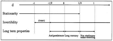
Fig. 1. Properties of a fractional integrated process

When 1/2<d<1, much work (Diebold and Rudebush 1991: 155–160) shows that the usual unit root tests display a bias in favour of the hypothesis ‘d = 1’. This is not very surprising because only the two cases d = {0,1} are considered in the ‘traditional unit-root’ framework. In contrast, the fractional framework allows a wider range of long-term patterns: all the cases . These processes are therefore very useful in the study of economic time series, which are known to display complicated long-term movements.

Hosking (1981: 165–176) demonstrated the fundamental properties of the ARFIMA(p,d,q) process. Asymptotically, these properties are given by those of the ARFIMA(0,d,0). Only the latter are presented here.

The stationary ARFIMA(0,d,0) process allows an infinite MA representation:

where (c₁ positive constant). The coefficients of MA(¥) development decay at a hyperbolic rate are different from the exponential rate characteristic of ARMA processes. The influence of a random shock will tend to vanish with time but at a relatively low speed.

The spectral density of the ARFIMA(0,d,0) process is:

where is the spectral density of the ARMA(p,q) process:

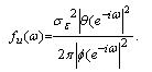
For (c₂ positive constant). The spectral density has a peak at zero frequency. Such a spectral shape is often connected with the presence of a non-stationary component. But the stationarity property is verified here. There is a risk of interpretation error when such a spectral shape is automatically associated with the non-stationarity of the series.

The algebraic expression of the ARFIMA(p,d,q) autocorrelation function is complex and of limited interest. Hosking (1981: 165–176) demonstrates that its asymptotic behaviour is (c₃ positive constant). One will find decay at a hyperbolic rate characteristic of fractional integrated processes.
It can be noted that if d>1/2, applying the first difference filter to the series, produces a series characterized by a fractional integration coefficient  for which one can verify: .

Then one can study differentiated series and deduce the properties of the raw series. Thus fractional integrated processes can model not only the phenomena of long memory but can also be used to implement a tool for time series analysis. For this, Beran (1999) proposes a model called SEMIFAR for the combined modelling of deterministic long-term trends (treated by a non-parametric approach) and stochastic long-term structures (processed by the parametric fractional model presented here).

2. An Overview of Estimation Techniques

2.1. Semiparametric Estimation

This method is used to estimate the value of the fractional integration coefficient by means of a simple procedure. The estimator is referred to as being ‘semiparametric’ because it does not assume a full parametric model for the short-term structure u_t but only a general hypothesis. It is assumed that the spectral density near zero frequency is . Long-term information is only used in the computation. In terms of spectral density, only frequencies near zero are used.

Obviously, the non-consideration of a possible short-term structure leads to a considerable risk of bias.

2.2. The Geweke and Porter-Hudak (GPH) estimator

After some transformations, the spectral density of the ARFIMA(p,d,q) process is:

where is the periodogram of the series x_t (estimator of the spectral density at the frequency .

If only the first m frequencies are used, with m such that , the influence of the short-term component can be considered constant and d can be estimated with a linear regression of from the deterministic regressor . It can be demonstrated that the estimator obtained is asymptotically normal and its variance is known (see Agikloglou, Newbold, and Wohar 1993: 235–246; Chen, Abraham, and Peiris 1994: 473–487; Cheung 1993: 331–345; Hassler 1994: 19–30; Hurvich and Ray 1995: 17–42; Reisen 1994: 335–350).[4]

A significance test of the fractional integration coefficient can be set up:

We note that in expression (7) the term is the asymptotic standard error of residuals in the regression discussed above.

This estimator can be improved if a smoothed periodogram is used instead of I_n(Hassler 1994: 19–30). Using a particular spectral window, Velasco (1999a: 325–371) proposes an estimator of d which can be used on non-stationary series. The author proves the consistency of this estimator for 1/2 < d < 1 and asymptotic normality for 1/2 < d < 3/4:[5]

2.3. Gaussian Semiparametric Estimator

This semiparametric estimator has been proposed by Robinson (1995: 1630–1661) and studied by Velasco (1999b: 87–127).

It belongs to the same logic as the GPH estimator but it is computed by minimization of the objective function Q(c,d):

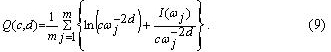
As for the GPH estimator, the use of a particular spectral window enables direct computation on series such that d<1 (Velasco 1999a: 87–127).

2.4. Fully Parametric Methods

These methods allow the simultaneous estimating of all the parameters of the process, the fractional integration coefficient and the parameters of an ARMA structure. They are based on the optimization of the likelihood function.

2.5. Exact Maximum Likelihood Estimator

The estimator of the exact maximum likelihood proposed by Sowell (1992: 165–188) is the vector .

It maximizes the log-likelihood function _L():

where R is the variance-covariance matrix of the process.

has an asymptotically normal distribution, and the variance matrix of parameters is given by the inverse of the information matrix.

The matrix R used in (8) is a complicated algebraic expression and is difficult to compute. Moreover, the exact maximum likelihood estimator may be biased if the mean of the series used is unknown.

2.6. Approximated Likelihood Estimators

We therefore use methods based on an approximation of the likelihood function.

The two main available techniques are the spectral approximation of Fox and Taqqu (1986: 517–532) and the minimization of the conditional sum of squared residuals proposed by Cheung and Baillie (1993: 791–806).

Asymptotically, these two methods converge on the exact maximum likelihood estimator.

The estimator suggested by Fox and Taqqu is the vector which maximizes the following expression:

 

This expression is easier to use but can display a bias in small samples. On the other hand, it is effective when the value of the mean of the process is unknown.

The estimator proposed by Cheung and Baillie is the vector  which minimizes the quantity:

This estimator can easily be modified to introduce an estimator of the mean into the parameter vector. It can be developed to take into account an heteroskedasticity in the residuals. But it can present a bias, particularly if the number of parameters is important or of it is performed in a small sample context.

The three estimators , and possess a normal asymptotic distribution for d<1/2, that is in the stationary case. No theoretical result exists that enables the computing of or directly on non-stationary series, as it is possible in the semiparametric case. Faced with non-stationarity, the only solution is to apply the first differences filter prior to performing the estimation. This removes all problems related to the presence of an unknown constant term (i.e. the mean of first differences is zero).

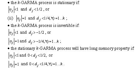
3. Generalization of Fractional Integration

In his paper, Hosking (1981: 165–176) notes that taking the fractional power of a second order polynomial makes it possible to describe long-term structures of periodic shape. Thus, Gray, Zang and Woodward (1989: 233–255) proposed the process called Generalized ARMA (GARMA). According to the values of the parameters, this process can possess a cyclical and persistent structure. Woodward, Chen and Gray (1998: 485–504) extended this model to the case in which the series have a k cyclical persistent component. The latter model is the most successful shape of fractional integration model.

Formally, the series x_{t, t=1..n} process if:

 

with the same notations as above; in particular, u_t is a stationary and inver-tible ARMA(p,q) process. Obviously, the model specification must be such that . The long-term structure now depends on two parameters. The parameter indicates the long-term periodicity while parameter d is linked to the ‘intensiveness’ of long-term structure. The quantity gives the periodicity in temporal terms. If , it can be verified that the cycle period tends toward infinity (the ARFIMA case).

It can be demonstrated that (Woodward, Chen, and Gray 1998: 485–504) that:

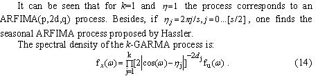
The spectral density shows k peaks at the frequencies . The estimation method proposed by Chung^[6] is based on the minimization of the conditional sum of squared residuals (noted CSS below).

However, parameter estimation of this class of process is delicate. In case k = 1, Chung shows that the estimator of obtained by CSS minimization converges at a greater speed than the other parameters. This rules out the use of gradient-based methods on the whole set of parameters.^[7] Therefore it is advisable to use an alternative method based on an incremental search (or grid-search). This method is very slow if the grid-search corresponds to [–1, 1]. It is then more effective to restrict the search interval to a neighborhood of frequencies relative to the strongest values of the periodogram. For k = 1, Chung demonstrates that the distribution of the estimators of d, as well as those of a possible ARMA structure obtained by minimization of the CSS function, is normal. Parameter significativity can be tested by a Student significance test. Moreover, the author shows that the law of parameter is known and proposes tabulated values ordinary to construct a confidence interval (Chung 1996a).

We pursue our analysis with the presentation of results stemming from our empirical study.

4. Empirical Study of Long-Term Structures for French Socio-Economic Series in the 19^th and 20^th Centuries

In this work, studied series are annual data observed over the period 1820–1996 for France (preceded by the letter F).

The used series are the GDP (GDP), the total population (POP), school population (SCOL), current (DECR) and constant (DECS) educational expenditures. Sources of series in levels are given in Diebolt et al. (2003).

A preliminary examination of the series shows:

1) a strong increase of all the series at the end of the observation period (from 1950) which will require transformation in logarithmic data. However, series are strongly non-stationary and the obtaining of coherent results is difficult.

2) the ‘evident non-stationarity’ of transformed series. The differences of size between the first and last observations leads to suspecting that the use of a model with a long memory runs into the problem of non-stationarity for series in levels.

The autocorrelation functions of level series display high and very weakly falling values. Periodograms are concentrated, with very low frequencies. Such observations first lead to developing a test of unit roots (Augmented Dickey and Fuller test). For reasons of conciseness detailed results are not presented here. We indicate, however, that for all the studied series, the hypothesis of unit root is easily accepted against an alternative of a deterministic trend. In some cases, the use of a test strategy of the Hénin-Jobert type leads to simultaneously accepting the presence of a unit root and a linear deterministic trend on first differences. This result may be at odds with intuition and, naturally, casts a doubt on the validity of the Dickey-Fuller test conclusions. The introduction of more elaborate alternatives, for example a trend with break, can lead to different results. Of course, the existence of a long-term structure can lead to a certain number of diagnosis errors (Diebold and Ruderbusch 1991: 155–160).

However that may be, our series of first differences present significant short term structures of varying length. At the same time, we note that the use of annual data results in diagnosis of a correlation structure is shorter than ten years as a short-term structure.

Statistical methods presented in the previous section are now used to discuss the shape of the long-term trends in the studied series. Two methods are investigated. We first envisage the presence of a long memory component with the use of ARFIMA processes. We seek then the presence of a cyclic long-term component with GARMA processes.

4.1. Search for Long Memory

The estimation method used here is a spectral approximation in the frequency domain (Fox and Taqqu 1986: 517–532). This algorithm requires starting va-lues close enough to the optimal values. In order to produce them, we compute first the GPH estimator and the results are used as the initial values in the optimization algorithm. The results are shown in Table 1.

Table 1. ARFIMA model estimation

Note: values in brackets give Student statistics.

The stationarization of the series was obtained with first differences and so it is advisable to add the value 1 to the numbers below to obtain the values of fractional integration coefficient for series in levels.

For France, all the coefficients are significantly different from zero, positive for all the series, except for FPOP. This result must be treated with caution because the GPH estimator is very sensitive to the presence of a short term component. Empirically, such a specification error can be suspected if the estimated values vary strongly when different number of ordinates are used in the periodogram regression (for different m or a). This seems to occur here.^[8] We verify that the orders of short term components are distinctly lower than those obtained after application of a first differences filter only. The maximum likelihood procedure confirms the previous results except for the FPOP series, which now displays a positive fractional integration coefficient. The short-term structure is now a MA(5) process for which the first and fifth terms are significant. The presence of a ‘troublemaker’ short term component seems confirmed. The FDECR series is very close to non-stationarity and presents no more short-term structures. All the series are persistent in first differences. The short-term components are low for FGDP and FSCOL, non-existent for FDECR and of order 5 for FPOP and FDECS.

The optimization procedure developed on the first differenciated series does not give any convergent results. The use of second differences gives an estimator close to –1/2. The raw series is therefore fractionally integrated of order approximately equal to 1.6 compared with the order 1.4 obtained in the French case. These two series are thus strongly non-stationary. Their correlation structures are largely formed by very long-term components that are difficult to exploit. This result underlines the difficulty of using current price data in a broad temporal framework. All the series show long memory behaviour linked to their slowness of adaptation to a shock. At such a level of aggregation, this result is not a surprise. Relatively close forms inside every country lead to considering that a long-term relation may exist among these variables. As a matter of fact, the similarities between the two countries lead us to thinking that the long-term evolution was driven by comparable determinants.

4.2. Long-Term Cycle Study

4.2.1. Single Component GARMA Model

Now we will try to go further in the search for a possible long-term component with finite periodicity. This study confirms the previous results (if the cycle frequency of the dominant long term component is infinite) or to complete them (if frequency is finite).

Indeed, the presence of a cycle with frequency close to zero but significantly different will mislead the estimation procedure of an ARFIMA process (overestimation of the short-term part). Furthermore, if we do not find such a cycle, checking the relation dARFIMA=2dGARMA obtained by two different optimization methods (spectral approximation of the log-likelihood function for ARFIMA and minimization of the sum of the squared conditional residuals for GARMA), makes it possible to confirm the results presented in the previous section. The results are shown in Table 2. No finite cycle appears as a dominant long-term structure. Coefficient h is not significantly different from 1 in all the series. All the series are persistent in differences. We verify the relationship linking the two fractional integration coefficients at least roughly. We retain a positive value for the fractional integration coefficient as well as a different short-term structure. Orders and values obtained for the short-term parameters are very close to the optimal values presented in Table 1. The slight differences results from a settlement between the value of coefficient
d and the variance of the residuals according to the two optimization methods.

Table 2. Single Component GARMA Estimation

4.2.2. Two-Component GARMA Model

To conclude this work, we present the results of the 2-GARMA model estimation. The estimated values of parameters for every series are shown in Table 3. The selection of the optimal short-term structure was made by repeating the estimation procedure for various values of the orders p and q and retaining as the optimal model that is relative to the minimal sum of squared
residuals.

First of all, we note that the method did not give stable results for the FPOP series (value 0 indicates that no model 2-GARMA could satisfactorily be fitted on this series). For these series the confidence interval of the parameter is equal to or is very close to the value 1. If there are effectively two fractional dynamics, they are too close for the method can not discriminate between them. On the contrary, everything seems to show that there is, for these series, only a single fractional component.

Table 3. 2-GARMA model estimation

Notes:

(i) The values printed in italics are those for which the nullity hypothesis is accepted, the values printed in bold italics are those for which a doubt remains. The values printed in bold are significant values.

(ii) The values in brackets give the Student statistic. The values in braces give the confidence interval obtained according to the values tabulated by Chung.

(iii) The sign ** indicates an algorithm failure to supply results.

For the other series, the value of the fractional integration coefficient for the parameter is fairly close to the value obtained by the estimation of the model 1-GARMA. This observation is evidence of the robustness of our result. The FGDP series present a persistent structure and a value of parameter corresponding respectively to a cycle of 7(,4) years and 13(,2) years. FDECR, FDECS and FSCOL series also seem to display a short-term structure but the fractional integration coefficient is not significant for these series.

However, the estimation results show that a gain in term of the sum of squared residuals is brought by the introduction of the second constituent.
A test with an acceptance probability of 10 % makes it possible to retain these variables. So one can accept the presence of a second long term structure with reserve. They would correspond to cycles of period 9(,8) years for FDECS, 9(,2) years for FDECR and 22 years for FSCOL.

A summary of the obtained results is given in the Table 4.

Table 4. Properties of the series

Series	Long-term structure	Long-term cycle	Short-term structure
FGDP	Unit root and long memory	13 years	1 year (AR)
FPOP	Unit root	none	5 years (MA)
FDECR	Unit root and long memory	9 years	none
FDECS	Unit root and long memory	20 years	5 years (AR)
FSCOL	Unit root and long memory	22 years	1 year (AR)

At the current state of knowledge, analysis by fractional integrated processes is the most appropriate method for describing the phenomena of long memory and, more widely, for identifying and/or clarifying certain theoretical hypotheses with view to modelling long-term cyclic movements.

At the point we have reached, it is therefore possible to shed light on the empirical results mentioned above. The cliometric analysis of educational series, economic growth and demography in France in the 19^th and 20^th centuries leads us to a significant result: no long-term cycle appears as the dominant constituent. Nevertheless, there are cycles which seem to affect some of the variables that we have studied. Others do not show any particular movement.

In Table 4, we distinguish first of all movements close to the classic cycle of the Juglar type (average duration of which is between 7 and 11 years) for the FGDP and FDECR series.

We then observe for FGDP, FPOP, FDECS and FSCOL series, cycles of 5 years or less; these are similar to minor cycles of the Kitchin type (average duration is 40 months).

We also note Kuznets type cycles in the FDECS and FSCOL series.
The latter found a periodicity of about 22 years for a period of a complete oscillation of production and 23 years for prices.

Finally, we have not noticed any cyclicity close to long movements such as Kondratieff cycles (whose average duration is between 48 and 60 years)
(Diebolt and Doliger 2006: 39–47; Metz 2011: 204–238).

As in the myth of Sisyphus, the boulder is at the bottom of the hill again!

References

Abramovitz M. 1965. The Nature and Significance of Kuznets Cycles. Readings in Business Cycles / Ed. by R. Aaron, and L. R. Klein, pp. 519–545. Homewood: Richard D. Irwin.

Agikloglou C., Newbold P., and Wohar W. 1993. Bias in the Estimator of the Fractional Difference Parameter. Journal of Time Series Analysis 14: 235–246.

Beran J. 1999. SEMIFAR Models – A Semiparametric Framework for Modelling Trends, Long Range Dependance and Non Stationarity. CoFE Discussion Paper 99–16. Konstanz: University of Konstanz.

Chen G., Abraham B., and Peiris S. 1994. Lag Window Estimation of the Degree of Differencing in Fractionally Integrated Time Series Models. Journal of Time Series Analysis 15: 473–487.

Cheung Y-W. 1993. Tests for Fractional Integration: A Monte-Carlo Investigation. Journal of Time Series Analysis 14: 331–345.

Chung C. F. 1996a. Estimating a Generalized Long Memory Process. Journal of Econometrics 73: 237–259.

Chung C. F. 1996b. A Generalized Fractionally Integrated Autoregressive Moving Average Process. Journal of Time Series Analysis 17: 111–140.

Chung C-F., and Baillie R. 1993. Small Sample Bias in the Conditional Sum of Squares Estimators of Fractionally Integrated ARMA Models. Empirical Economics 18: 791–806.

Diebold F.,and Rudebush G. 1991. On the Power of Dickey–Fuller Tests against Fractional Alternatives. Economics Letters 35(2): 155–160.

Diebolt C., and Doliger C. 2006. Economic Cycles under Test: A Spectral Analysis. Kondratieff Waves. Warfare and World Security/ Ed. by T. Devezas, pp. 39–47. Amsterdam: IOS Press.

Diebolt C., Guiraud V., and Monteils M. 2003. Education, Knowledge and Economic Growth. France and Germany in the Nineteenth and Twentieth Centuries. Frankfurt am Main: Peter Lang.

Fox R.,and Taqqu M. 1986. Large Sample Properties of Parameters Estimates for Strongly Dependent Stationary Gaussian Time Series. The Annals of Statistics 14: 517–532.

Granger C., and Joyeux R. 1980. An Introduction to Long Memory Time Series and Fractional Differencing. Journal of Time Series Analysis 1: 1–15.

Gray H., Zang N., and Woodward W. 1989. On Generalized Fractional Processes. Journal of Time Series Analysis 10: 233–257.

Hassler U. 1994. (Mis)specification of Long Memory in Seasonal Time Series. Journal of Time Series Analysis 15: 19–30.

Heinrich W. 1928. Grundlagen einer universalistischen Krisenlehre. Jena: G. Fischer.

Hosking J. 1981. Fractional Differencing. Biometrika 68: 165–176.

Hurst H. 1957. A Suggested Statistical Model for Some Time Series that Occur in Nature. Nature 180: 494.

Hurvich C., and Ray B. 1995. Estimation of the Memory Parameter of Nonstationary or Non-Invertible Fractionally Integrated Process. Journal of Time Series Analysis 16(1): 17–42.

Imbert G. 1959. Des mouvements de longue durée Kondratieff. Aix-en-Provence: La pensée universitaire.

Juglar C. 1889. Des crises commerciales et de leur retour périodique en France, en Angleterre et aux Etats-Unis. Paris: Guillaumin et Cie.

Kleinknecht A. 1987. Innovation Patterns in Crisis and Prosperity. Schumpeter's Long Cycle Reconsidered. London: The Macmillan Press Ltd.

Kondratieff N.D. 1926. Die langen Wellen der Konjunktur. Archiv für Sozialwissenschaft und Sozialpolitik 56: 573–609.

Kuznets S. 1930. Secular Movements in Production and Prices. Their Nature and their Bearing upon Cyclical Fluctuations. Boston, MA: Houghton Mifflin Co.

Mandelbrot B., and Van Ness J.W. 1968. Fractional Brownian Motion, Fractional Brownian Noise and Applications. SIAM Review 10: 422–437.

Mensch G. 1977. Das technologische Patt. Innovationen überwinden die Depression. Frankfurt am Main: Fischer Taschenbuch Verlag.

Metz R. 2011. Do Kondratieff Waves Exist? How Time Series Techniques Can Help to Solve the Problem. Cliometrica 5: 204–238.

Odaki M. 1993. On the Invertibility of Fractionally Differenced ARIMA Processes. Biometrika 80: 703–709.

Petzina D., and Roon G. van. (Eds.) 1981. Konjunktur, Krise, Gesellschaft. Wirtschaftliche Wechsellagen und soziale Entwicklung im 19. und 20. Jahrhundert. Stuttgart: Klett-Cotta.

Reisen V. 1994.Estimation of the Fractional Difference Parameter in the ARIMA(p,d,q) Model Using the Smoothed Periodogram. Journal of Time Series Analysis 15: 335–350.

Robinson P. 1995. Gaussian Semiparametric Estimation of Long Range Dependance. The Annals of Statistics 23(5): 1630–1661.

Salin E. 1929. Geschichte der Volkswirtschaftslehre. Berlin: J. Springer.

Schumpeter J.A. 1939. Business Cycles. A Theoretical, Historical and Statistical Analysis of the Capitalist Process. 2 vols. New-York – Toronto – London: McGraw-Hill Book Co.

Sowell F. 1992. Maximum Likelihood Estimation of Stationary Univariate Fractionally Integrated Time Series Model. Journal of Econometrics 53: 165–188.

Velasco C. 1999a. Non-stationary Log-Periodogram Regression. Journal of Econometrics 91: 325–371.

Velasco C. 1999b. Gaussian Semiparametric Estimation of Non-Stationary Time Series. Journal of Time Series Analysis 20: 87–127.

Wagenführ R. 1929. Die Konjunkturtheorie in Russland. Jena: G. Fischer.

Weinstock U. 1964. Das problem der Kondratieff-Zyklen. Ein Beitrag zur Entwicklung einer Theorie der ‘langen Wellen’ und ihrer Bedeutung. Berlin: Duncker & Humblot.

Woodward W., Chen Q.,and Gray H. 1998. A K-Factor GARMA Long-Memory Model. Journal of Time Series Analysis 19(4): 485–504.

Woytinsky W. 1931. Das Rätsel der langen Wellen. Schmollers Jahrbuch für Gesetzgebung, Verwaltung und Volkswirtschaft im Deutschen Reich 55: 1–42.