The 21st Century Singularity in the Big History Per-spective. A Re-analysis

Download

DOI: https://doi.org/10.30884/978-5-7057-6469-3_04 

Abstract

The idea that in the near future we should expect ‘the Singularity’ has become quite popular recently, primarily thanks to the activities of Google technical director in the field of machine training Raymond Kurzweil and his book The Singularity Is Near (2005). It is shown that the mathematical analysis of the series of events (described by Kurzweil in his famous book), which starts with the emergence of our Galaxy and ends with the decoding of the DNA code, is indeed ideally described by an extremely simple mathematical function (not known to Kurzweil himself) with a singularity in the region of 2029. It is also shown that, a similar time series (beginning with the onset of life on Earth and ending with the information revolution – composed by the Russian physicist Alexander Panov completely independently of Kurzweil) is also practically perfectly described by a mathematical function (very similar to the above and not used by Panov) with a singularity in the region of 2027. It is shown that this function is also extremely similar to the equation discovered in 1960 by Heinz von Foerster and published in his famous article in the journal ‘Science’ – this function almost perfectly describes the dynamics of the world population and is characterized by a mathematical singularity in the region of 2027. All this indicates the existence of sufficiently rigorous global macroevolutionary regularities (describing the evolution of complexity on our planet for a few billions of years), which can be surprisingly accurately described by extremely simple mathematical functions. At the same time it is demonstrated that in the region of the singularity point there is no reason, after Kurzweil, to expect an unprecedented (many orders of magnitude) acceleration of the rates of technological development. There are more grounds for interpreting this point as an indication of an inflection point, after which the pace of global evolution will begin to slow down systematically in the long term.

Keywords: universal evolution, global evolution, Big History, hyperbolic growth, Singularity.

Introduction

The issue of the Global History singularity (or even the Big History singularity) is being discussed rather actively nowadays (see, e.g., Eden et al. 2012; Shanahan 2015; Callaghan 2017; Nazaretyan 2015a, 2016, 2017, 2018). This subject has been made especially popular by Raymond Kurzweil, Google technical director in the field of machine training, first of all with his book The Singularity Is Near (2005), but also with such activities as the establishment of the Singularity University (2009) and so on. The issue of Singularity was brought into the realm of Big History by such Big Historians as Akop Nazaretyan (2005a, 2005b, 2009, 2013, 2014, 2015a, 2015b, 2016, 2017, 2018; see also Nazaretyan 2020: Ch. 15), Alexander Panov (2004, 2005a, 2005b, 2006, 2008, 2011, 2017; see also 2020: Ch. 20), and Graeme Donald Snooks (2005; see also 2020: Ch. 12). In the Big History perspective, the ‘Singularity Hypothesis’ might be of some interest, as it virtually suggests a rather exact dating of the onset of Big History Threshold 9 (around 2045 CE). However, let us find out if those calculations of the Singularity timing can indeed be used to identify the possible date of the nearest Big History threshold.

Kurzweil – Modis Time Series
and Mathematical Singularity

Raymond Kurzweil was one of the first to arrange the major evolutionary shifts of a very significant part of the Big History along the hyperbolic curve that can be described by an equation with a mathematical singularity. For example, in his bestseller The Singularity Is Near (2005: 18) he reproduces the following figure (see Fig. 1)^[1].

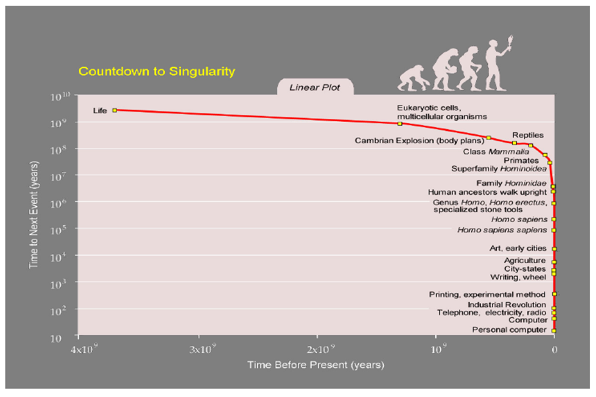
Fig. 1. ‘Countdown to Singularity’ according to Raymond Kurzweil

Source: Kurzweil 2005: 18 (reproduced with permission of Raymond Kurzweil).

However, rather surprisingly, Kurzweil does not appear to have recognized that the curve represented at this figure is hyperbolic, and that it is described by an equation possessing a true mathematical singularity (what is more the value of this singularity, 2029 is not so far from the one professed by Kurzweil himself). This appears to be explained first of all by some mathematical inaccuracies of the Google technical director (suffice to mention that he consistently calls the global evolution acceleration pattern ‘exponential’ without paying attention to the point that the exponential function does not have any singula-
rity).

Against this background, it appears a bit surprising that Kurzweil himself does know about the notion of mathematical singularity and describes it more or less accurately. Indeed, in his bestseller he provides a fairly accurate description of the concept of ‘mathematical singularity’:

To put the concept of Singularity into further perspective, let's explore the history of the word itself. ‘Singularity’ is an English word meaning a unique event with, well, singular implications. The word was adopted by mathematicians to denote a value that transcends any finite limitation, such as the explosion of magnitude that results when dividing a constant by a number that gets closer and closer to zero. Such a mathematical function never actually achieves an infinite value, since dividing by zero is mathematically ‘undefined’ (impossible to calculate). But the value of y exceeds any possible finite limit (approaches infinity) as the divisor x approaches zero (Kurzweil 2005: 22–23).

What is more, he supplies his description of the concept of ‘mathematical sin-
gularity’ with a rather appropriate illustrating diagram (see Fig. 2).

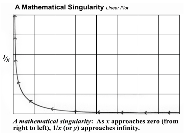
Fig. 2. A mathematical singularity

Source: Kurzweil 2005: 23 (reproduced with permission of Raymond Kurzweil).

However, having provided his fairly adequate description of the mathematical singularity concept, Kurzweil appears to be losing any interest in this concept – suddenly switching to the use of the term ‘singularity’ by astrophysicists (Ibid.).

One of the most enigmatic things in Kurzweil's book is that he manages not to notice that the shape of the hyperbolic curve at his figure ‘A mathematical singularity’ (Kurzweil 2005: 23; see also Fig. 2 above) is fundamentally identical (though, of course, rotated 180 degrees) with the one of the curve of his figure ‘Countdown to Singularity’ (Ibid.: 18, see Fig. 1 above). What is more, as we will see below, the mathematical model providing the best-fit approximation of the curve of the type seen in Fig. 1 is basically identical with the hyperbolic function displayed in Fig. 2, that is y = k/x. Thus, if Kurzweil had done a basic mathematical analysis of the time series in his Fig. 1, he would have found that it is best described by a mathematical equation of the type he features in
his Fig. 2 (with such a really slight difference that we would have ‘2’ rather than
‘1’ in the equation's numerator^[2]). What is more, he would have discovered that the mathematical singularity of the best-fit equation describing Kurzweil's ‘Countdown to Singularity’ curve is 2029, which is not so much different from 2045, suggested by him in his book, and that is simply identical with the date proposed by Kurzweil most recently (Ranj 2016).^[3]

Panov’s Transformation

Another amazing thing is that what was not done by Kurzweil in 2005, was done in 2003 by Alexander Panov^[4] who analyzed an essentially similar time series taken from entirely different sources but arrived at very similar conclusions, but in a much more advanced form. It is very important that he made a step (to which Kurzweil was very close but which he did not make actually) that allowed him to make the analysis of the time series in question much more transparent and to identify the singularity date in a rigorous way.

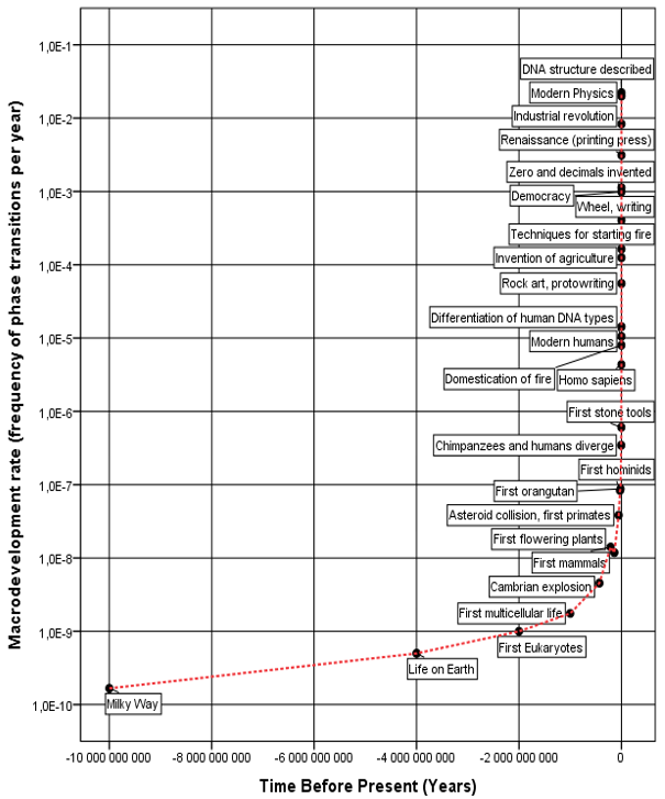
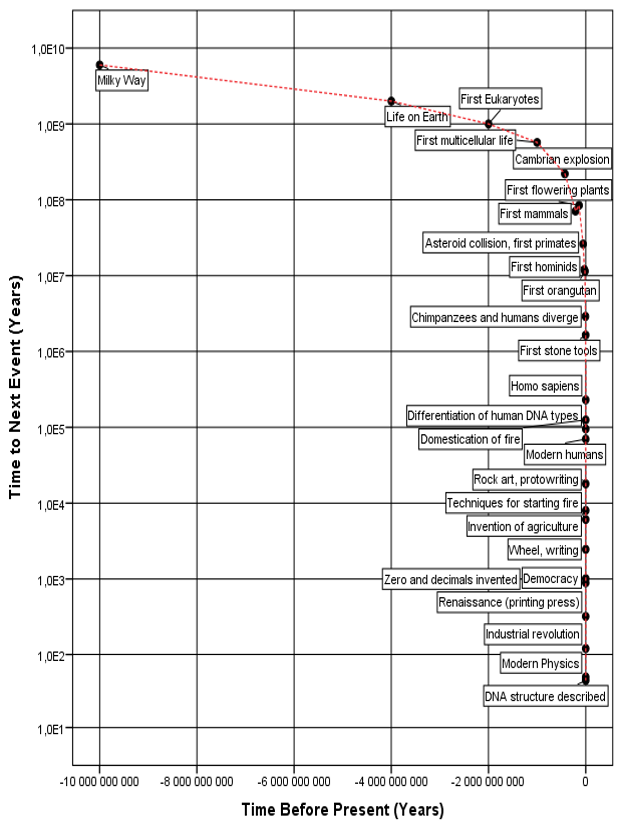
In his 2005 book Kurweil plotted at the Y-axis of his diagrams ‘time to next event’, which hindered for him their interpretation in a rather significant way. In his 2001 essay at page 5 while analyzing a diagram with a similar time series (whose source, incidentally, was not indicated), Kurzweil noted the acceleration of ‘paradigm shift rate’ (Kurzweil 2001: 5), but (as is rather typical for the Google Chief Engineer) almost immediately switched to another theme. However, what was necessary to make his diagrams much more intelligible was to plot at Y-axis not ‘Time to Next Event’, but just ‘Paradigm Shift Rate’ – just as was done by Panov. Indeed, to transform the time to next paradigm shift into paradigm shift rate one needed to do a rather simple thing – to take one year and to divide it by time to next paradigm shift; this will yield number of paradigm shifts per year, that is just a ‘Paradigm Shift Rate’. As we have already said, this was not done by Kurzweil but was done by Panov who obtained the following graphs as a result (see Fig. 3).

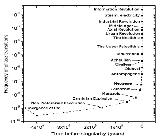
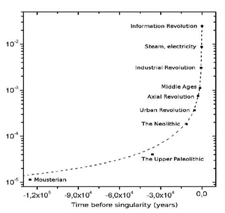
Fig. 3. The dynamics of the global macrodevelopment rate according to Panov

Source: Nazaretyan 2018: 31, Fig. 3.

The left-hand diagram in Fig. 3 shows the acceleration of the global macroevolution rate starting from 4 billion BP, whereas the right-hand diagram describes this for the human part of the Big History.^[5] Note immediately that Panov's left-hand curve in Fig. 3 is a mirror image of Kurzweil's ‘Countdown to Singularity’ graph (see Fig. 4).

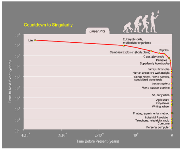
Fig. 4. Comparison between Kurzweil’s ‘Countdown to Singularity’ and Panov’s graphic depiction of the dynamics of the ‘frequency of global phase transitions’ (= global macroevolution rate)

However, the mathematical interpretation of Panov's graph is much easier and more straightforward. Note that Panov himself denoted the variable plotted at Y-axis as ‘Frequency of the phase transitions per year’. However, it is quite clear that Panov's ‘phase transition’ is a synonym of Kurzweil's ‘paradigm shift’, whereas ‘frequency of the phase transitions per year’ describes just ‘paradigm shift rate’, or global evolutionary macrodevelopment rate. This transformation makes it much easier to detect rigorously the pattern of acceleration of the global macrodevelopment rate.

Modis – Kurzweil Time Series:
A Mathematical Analysis

Below we will perform a mathematical analysis of Kurzweil's time series along the lines suggested by Panov (though with some modifications of ours).

In addition to Kurzweil's ‘Countdown to Singularity’ graph in single logarithmic scale presented above at Fig. 1, Kurzweil publishes two other versions of this graph in double logarithmic scale (see Figs. 5 and 6):

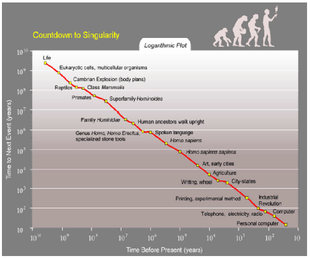
Fig. 5. The first log-log version of Kurzweil’s ‘Countdown to Singularity’ graph

Source: Kurzweil 2005: 17 (reproduced with permission of Raymond Kurzweil).

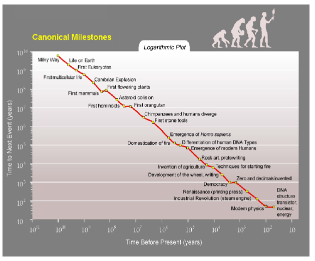
Fig. 6. The second log-log version of Kurzweil’s ‘Countdown to Singularity’ graph (= ‘Canonical Milestones’)

Source: Kurzweil 2005: 20 (reproduced with permission of Raymond Kurzweil).

Though the time series presented in Fig. 5 looks for me a bit more convincing than the one presented in Fig. 6, I have decided to analyze the time series in Fig. 6 due to the following reason. The point is that the source of data for Fig. 5 remains entirely obscure; hence, I do not see any way to reconstruct the respective time series in such a detail that is necessary for its formal mathematical analysis. There are no such problems with the source of data for Fig. 6, as Kurzweil indicates it very clearly. This is a paper by Theodore Modis The Limits of Complexity and Change (2003) prepared in turn on the basis of his earlier article published in Technological Forecasting and Social Change (2002). Fortunately, Modis provides all the necessary dates in his articles, which makes it perfectly possible to analyze this time series mathematically.

We will start our analysis with the abovementioned transformation, i.e. replace ‘time to next event’ with ‘paradigm shift rate’ ~ ‘phase transition rate’ ~ ‘macrodevelopment rate’. The result looks as follows (see Fig. 7):

Fig. 7. Kurzweil’s ‘Canonical Milestones’ graph^[6] transformed with Panov’s technique (single logarithmic scale)

Applying the same technique (‘Countdown to Singularity’) as the one used by Kurweil for Fig. 1, we would obtain for this time series the following graph (see Fig. 8).

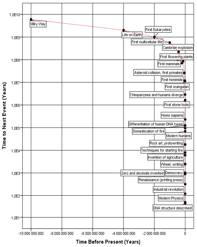
Fig. 8. Kurzweil’s ‘Canonical Milestones’ graph^[7] with single logarithmic scale

In Fig. 9 we can see that one figure is an exact mirror image of the other (see Figs. 9a and 9b).

It can be clearly seen that the curve in Fig. 7 (= Fig. 9a) is virtually the same as the hyperbolic one in Fig. 2 representing the mathematical singularity. At the next step let the X-axis represent the time before the singularity (whereas the Y-axis will represent the macrodevelopment rate) – and calculate the singularity date by getting such a power-law curve that would describe our time series in the most accurate way. The results of this analysis are presented in Fig. 10 (as has been mentioned above, our mathematical analysis has identified the Singularity date for this time series as 2029 CE).

(a)

(b)

Fig. 9. ‘Panov’s’ diagram (a) is a mirror image of ‘Kurzweil’s’ (b) one

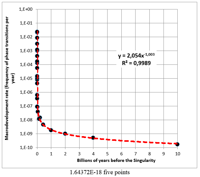
Fig. 10. Scatterplot of the phase transition points from the Modis – Kurzweil list with the fitted power-law regression line (with a logarithmic scale for the Y-axis) – for the Singularity date identified as 2029 CE with the least squares method

Below the same figure is presented in the double logarithmic scale (see Fig. 11).

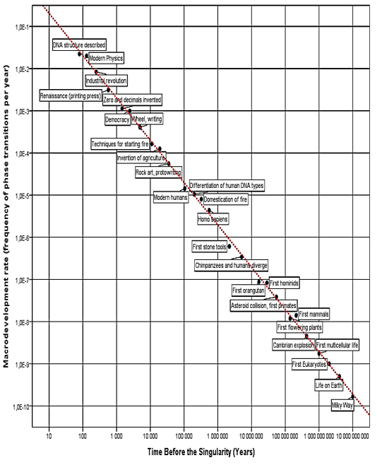
Fig. 11. Scatterplot of the phase transition points from the Modis – Kurzweil list with the fitted power-law regression line (double logarithmic scale) – for the Singularity date identified as 2029 CE with the least squares method

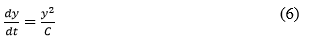
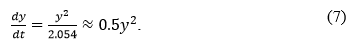
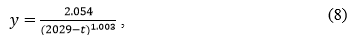
Let us now analyze the results. As we see, Kurzweil time series is described precisely with a mathematical function of a type y = k/x having an explicit mathematical singularity that was described by Kurzweil in his book (Kurzweil 2005: 22–23) surprisingly without understanding of its relevance for the mathematical description of the ‘Countdown to Singularity’ time series presented by him just a few pages before (Ibid.: 17–20). Indeed, our power-law regression of the last ‘Countdown to Singularity’ time series has identified the following best fit equation describing this time series in an almost ideally accurate (R² = 0.999) way:

where y is the global macrodevelopment rate, x is the time remaining till the singularity, and 2.054 and 1.003 are constants.

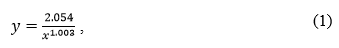
Note that the denominator's exponent (1.003) turns out to be only negligibly different from 1 (well within the error margins); hence, there are all grounds to use this equation in the following simplified form:

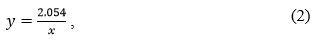
where y is the global macrodevelopment rate, x is the time remaining before the Singularity, and 2.054 is a constant.

Thus, we find out that the Kurzweil – Modis data series is the best described mathematically just by a simple hyperbolic function of that very type that he presents at pages 22–23, with the only difference that it has 2 (rather than 1) in the numerator.^[8]

Exponential and Hyperbolic Patterns
of Global Acceleration: A Comparison

Let us stress again that the mathematical analysis demonstrates rather rigorously that the development acceleration pattern within Kurzweil's series is NOT exponential (as is claimed by Kurzweil), but hyperexponential, or, to be more exact, hyperbolic (see Fig. 12).

Let us recollect that, with a logarithmic scale for the Y-axis, an exponential curve looks like a straight line (whereas a hyperbolic line looks like an exponential curve). On the other hand, in double logarithmic scale the hyperbolic curve looks like a straight line, whereas the exponential curve looks like an inversed exponential line. Thus, Fig. 12 demonstrates how wrong Kurzweil is when he claims that megaevoluton has followed the exponential acceleration pattern, indicating that this pattern was not exponential but hyperbolic.

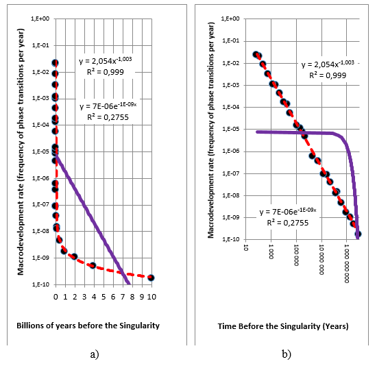
Fig. 12. Scatterplot of the phase transition points from the Modis – Kurzweil list with fitted power-law/hyperbolic and exponential regression lines: a) with a logarithmic scale for the
Y-axis; b) double logarithmic scale. Solid curves have been generated by the best-fit exponential model, whereas dashed curves have been generated by the hyperbolic equation

Formula of Acceleration of the Global
Macroevolutionary Development
in the Modis – Kurzweil Time Series

To make the model more transparent, it makes sense to make a small transformation of Eq. (2). Let us recollect that this is a slightly simplified version of Eq. (1) that was used to generate the hyperbolic curves at Fig. 12 above, and it looks as follows:

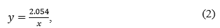
where y is the global macrodevelopment rate, x is the time remaining before the singularity, and 2.054 is a constant.

Of course, x (the time remaining till the singularity) at the moment of time t equals t* – t, where t* is the time of singularity. Thus,

х = t* – t.

Hence, Eq. (2) can be rewritten in the following way:

where y_t is the global macrodevelopment rate at time t, t* is the time of singularity, and 2.054 is a constant.

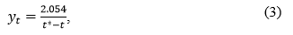
Finally, let us recollect that our least squares analysis of the transformed Modis – Kurzweil series has identified the singularity date as 2029 CE. Thus, Eq. (3) can be further rewritten in the following way:

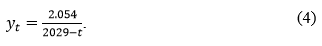
Of course, in a more general form it should be written as follows:

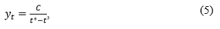
where C and t* are constants.

Eq. (4) generates curves that demonstrate an extremely accurate fit with empirical estimates and that are presented in Figs. 13–15 below.

The curve generated by this extremely simple equation describes in an unusually accurate way the planetary macroevolution acceleration pattern at the scale of billions of years (see Fig. 13).

However, if we ‘zoom in’ Fig. 13 to see in more detail the recent two billions of years, we will see that Eq. (4), notwithstanding its extreme simplicity, turns out to be as capable to describe rather accurately the planetary macroevolution acceleration pattern (see Fig. 14).

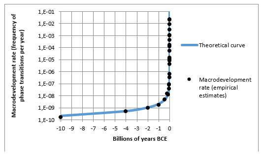
Fig. 13. Fit between the empirical estimates of the macrodevelopment rate and the theoretical curve generated by the hyperbolic equation y_t = 2.054/(2029 – t), 10 billion BCE – 2000 CE, with a logarithmic scale for the Y-axis

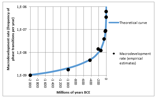
Fig. 14. Fit between the empirical estimates of the macrodevelopment rate and the theoretical curve generated by the hyperbolic equation y_t = 2.054/(2029 – t), 2 billion – 2 200 000 BCE, with a logarithmic scale for the Y-axis

If we zoom in further – to see in some detail the global macroevolutionary development acceleration during the last hundreds of thousands of years of Big History (corresponding to the pre-history and history of the humankind) we will see a similarly astonishingly close fit between the curve generated by model (4) and the empirical estimates of the global macroevolution rate (see Fig. 15).

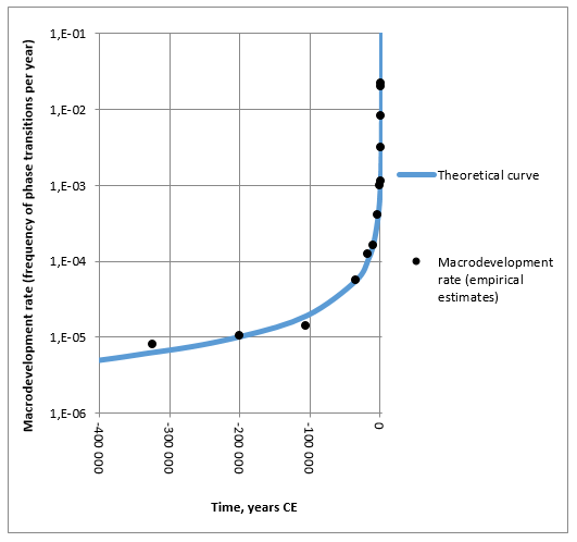
Fig. 15. Fit between the empirical estimates of the macrodevelopment rate and the theoretical curve generated by the hyperbolic equation y_t = 2.054/(2029 – t), 400 000 BCE – 2000 CE, with a logarithmic scale for the Y-axis

Finally, if we concentrate on the last millennia of the ‘human history’ phase of the Big History, we will see that the same equation describes them as accurately (see Fig. 16).

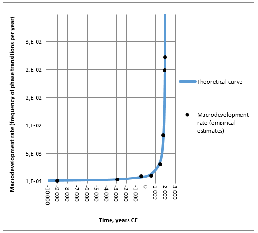
Fig. 16. Fit between the empirical estimates of the macrodevelopment rate and the theoretical curve generated by the hyperbolic equation y_t = 2.054/(2029 – t), 10 000 BCE – 2000 CE, with a natural scale for the both axes

I would stress again that the curve accurately describing the acceleration of human history after 10 BCE (Fig. 16) and the curve as accurately describing the acceleration of planetary macroevolution before the appearance of humans have been generated by the same equation – the simplest Eq. (4).

As we see, a very simple hyperbolic equation y_t = 2.054/(2029 – t) describes the general pattern of the macrodevelopment rate acceleration observed up until recently in an extremely accurate way for all the main eras.

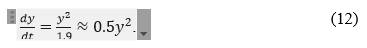
In fact, Model (4) has a rather straightforward ‘physical sense’. Indeed, let us calculate the macroevolution rate around 200 years before the ‘Singularity’ (that is around 1829) using this equation in a further simplified form (y_t = 2/(2029 –
– t)): y₁₈₂₉ = 2/(2029 – 1829) = 2/200 = 1/100. Thus, we arrive at the following result: ‘around 1800 CE a typical rate of global macroevolution was about one macroevolutionary shift (e.g., Industrial Revolution) per century’ – that is macroevolution around that time proceeded at the scale of centuries.

The same calculations for the time point about 2,000 years before the Singularity (≈ before present) – around 1 CE in 29 CE would yield the following result: y₂₉ = 2/(2029–29) = 2/2000 = 1/1000 – that is macroevolutionary shifts (e.g., Axial Age revolution) tended to happen at the scale of one per millennium and the evolution proceeded at that time at the scale of millennia. On the other hand, around 18 000 BCE we would find that planetary macroevolution occurred at the scale of tens of thousands of years, around 200 000 years before present (BP) – at the scale of hundreds thousands of years (around one global phase transition per 100 thousand years), around 2 million BP – at the scale of millions of years, around 20 million BP – at the scale of tens of millions of years, around 200 million BP – at the scale of hundreds of millions of years, and around 2 billion BP – at the scale of billions of years (that is, approximately one planetary macroevolutionary phase transition per one billion of years). In other words, with every decrease of the time to present (≈ to the ‘Singularity’) by an order of magnitude (from 2 billion BP to 200 million BP, from 200 million BP to 20 million BP, from 20 million BP to 2 million BP, etc.) the rate of global macroevolutionary development every time also increased just by an order of magnitude. And for me such an acceleration pattern makes a perfect sense.

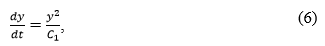
Note that algebraic equation of the type

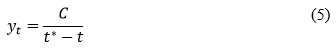
can be regarded as solution of the following differential equation:

(see, e.g., Korotayev, Malkov, and Khaltourina 2006a: 118–120).

Thus, the acceleration pattern implied by Eq. (4) can be spelled out as follows:

Verbally, the overall pattern of acceleration of planetary macroevolution that describes so accurately the Modis – Kurzweil series of ‘complexity jumps’ with model (4) / (5) can be spelled out as follows: ‘the increase in macroevolutionary development rate a times is accompanied by a² increase in the accelerati-on speed of this development rate; thus, a twofold increase in macroevolutionary development rate tends to be accompanied by a fourfold increase in the acceleration speed of this development rate; an increase in macroevolutionary deve-
lopment rate 10 times tended to be accompanied by 100 times increase in the acceleration speed of this development rate; and so on…’.

Now, let us apply a similar methodology to analyze mathematically the series of global macroevolutionary ‘phase transition’/ ‘biospheric revolutions’ compiled by Alexander Panov (2005a, 2005b; see also Panov 2008, 2011, 2017).

However, before we do this I would like to analyze a few points.

Time Series of Panov and Modis – Kurzweil:
An External Comparative Analysis

Alexander Panov and Theodore Modis compiled their time series entirely independently of each other. As my personal communications with both Panov and Modis show, none of them knew that at almost the same time^[9] in another part of Europe another person compiled a similar time series (Alexander Panov worked in Moscow, whereas Theodore Modis worked in Geneva). As we will see below, they relied on entirely different sources and the resultant time series turned out to be very far from being identical.

Indeed the Modis time series (2003) standing behind Kurzweil's ‘Canonical Milestones’ graph (Kurzweil 2005: 20) looks as follows – we reproduce below this time series as it was published in Modis' essay in The Futurist (2003), as it is this version of Modis' series that is reproduced by Kurzweil and that has been analyzed mathematically above; however, we sometimes use fuller versions of the description of some Modis ‘milestones’ from his 2002 article in Technological Forecasting & Social Change:

(1)    Origin of Milky Way, first stars – 10 billion years ago.^[10]

(2)    Origin of life on Earth, formation of the solar system and the Earth, oldest rocks – 4 billion years ago.

(3)    First eukaryotes, invention of sex (by microorganisms), atmospheric oxygen, oldest photosynthetic plants, plate tectonics established – 2 billion years ago.

(4)     First multicelluar life (sponges, seaweeds, protozoans) – 1 billion years ago.

(5)    Cambrian explosion/invertebrates/vertebrates, plants colonize land, first trees, reptiles, insects, amphibians – 430 million years ago.

(6)    First mammals, first birds, first dinosaurs – 210 million years ago.

(7)    First flowering plants, oldest angiosperm fossil – 139 million years ago.

(8)    First primates/asteroid collision/mass extinction (including dinosaurs) – 54.6 million years ago.

(9)    First hominids, first humanoids – 28.5 million years ago.

(10)  First orangutan, origin of proconsul – 16.5 million years ago.

(11)  Chimpanzees and humans diverge, earliest hominid bipedalism – 5.1 million years ago.

(12)  First stone tools, first humans, Homo erectus – 2.2 million years ago.

(13)  Emergence of Homo sapiens – 555,000 years ago.

(14)  Domestication of fire / Homo heidelbergensis – 325,000 years ago.

(15)  Differentiation of human DNA types – 200,000 years ago.

(16) Emergence of ‘modern humans’/earliest burial of the dead – 105,700 years ago.

(17)  Rock art/ptotowriting – 35,800 years ago.

(18)  Techniques for starting fire – 19,200 years ago.

(19)  Invention of agriculture – 11,000 years ago.^[11]

(20)  Discovery of the wheel/writing/archaic empires/large civilizations/Egypt/
Mesopotamia – 4,907 years ago

(21)  Democracy/city states/Greeks/Buddha [≈ Axial Age] – 2,437 years ago.

(22)  Zero and decimals invented, Rome falls, Moslem conquest – 1,440 years ago.

(23)  Renaissance (printing press)/discovery of New World/the scientific method – 539 years ago

(24)  Industrial revolution (steam engine)/political revolutions (French, USA) – 225 years ago.

(25)  Modern physics/radio/electricity/automobile/airplane – 100 years ago.

(26)  DNA structure described/transistor invented/nuclear energy/WWII/Cold War/Sputnik – 50 years ago.

(27)  Internet/human genome sequenced – 5 years ago.

* Note that Modis himself maintains rather explicitly that ‘present time is taken as year 2000’ (Modis 2003: 31). Indeed, this makes good sense for ‘milestones’ (24)–(27) above. However, there are some indications that Modis compiled first versions of his milestone list a few years before 2000, and appears not to have adjusted a few datings to the 2000 present point in his 2003 publication. Otherwise it is difficult to understand his datings of milestones (20), (21), and (23).

Table 1. Comparison of sources used by Modis (2002, 2003) and Panov (2005a) for the compilation of their lists of phase transitions / ‘biospheric revolutions’ / ‘canonical milestones’ / ‘evolutionary turning points’ / ‘complexity jumps’

Thus, Modis (2002: 393–401) indicates the following list of sources he consulted to compile the time series above: Barrow and Silk 1980; Burenhult 1993; Heidmann 1989; Johanson and Edgar 1996; Sagan 1989; Schopf 1991; to this Modis also adds ‘Timeline of the Universe’ (American Museum of Natural History, Central Park West at 79^th Street, New York), Encyclopedia Britannica,^[13] ‘the web site of the Educational Resources in Astronomy and Planetary Science (ERAPS), University of Arizona’,^[14] ‘Private communication, Paul D. Boyer, Biochemist. Nobel Prize 1997. Dec 27, 2000’, ‘a timeline for major events in the history of life on earth as given by David R. Nelson, Department of Biochemistry at the University of Memphis, Tennessee’[15] (see Table 1 above).

On the other hand, Panov relied on entirely different sources^[16] (see Table 1 above).

As we see, there was not a single source consulted by both Modis (2002, 2003) and Panov (2005a) when they compiled their series of ‘canonical milestones / biospheric revolutions’. Their reference lists are 100 % different. What is more, they mostly relied on sources belonging to different scientific traditions. Indeed, Modis relied exclusively on the works of Western scientists published in English.^[17] In a striking contrast with this, out of 30 references consulted by Panov (2005a), 18 are works of Russian scientists published in Russia; 9 are works of Western scientists translated into Russian; and just three references are original works of Western scientists in English.

Against this background, it is hardly surprising that Panov's list of phase transitions (2005a: 124–127; 2005b: 221) has turned out to be very far from identical with the one of Modis:^[18]

‘0. The origin of life – 4 · 10⁹ years ago. The biosphere after its appearance was represented by nucleusless procaryotes and existed the first 2–2.5 billion years without any great shocks.

1. Neoproterozoic revolution (Oxygen crisis) – 1.5 · 10⁹ years ago. Cyanobacteria had enriched the atmosphere by oxygen that was a strong poison for anaerobic procaryotes. Anaerobic procaryotes started to die out and anaerobic procaryote fauna was changed by an aerobic eucaryote and multicellular one.

2. Cambrian explosion (The beginning of Paleozoic era) – 590–510 · 10⁶ years ago.^[19] All the modern phyla of metazoa (including vertebrates) appeared during a few of tens of million years. During the Paleozoic era the terra firma was populated by life.

3. Reptiles revolution (The beginning of Mesozoic era) – 235 · 10⁶ years ago. Almost all paleozoic Amphibia died out. Reptiles became the leader of the evolution on the terra firma.

4. Mammalia revolution (The beginning of the Cenozoic era) – 66 · 10⁶ years ago. Dinosaurs died out. Mammalia animals became the leader of the evolution on the terra firma.

5. Hominoid revolution (The beginning of the Neogene period) – 25–20 · 10⁶ years ago.^[20] A big evolution explosion of Hominoidae (apes). There were 14 genera of hominoidae between 22 and 17 million years ago – much more than now. The flora and fauna became contemporary.

6. The beginning of Quaternary period (Anthropogene) – 4.4 · 10⁶ years ago.^[21] The first primitive Homo genus (hominidae) separated from hominoidae.

7. Palaeolithic revolution – 2.0–1.6 · 10⁶ years ago.^[22] Homo habilis, the first stone implements.

8. The beginning of Chelles period – 0.7–0.6 · 10⁶ years ago.^[23] Fire, Homo erectus.

9. The beginning of Acheulean period – 0.4 · 10⁶ years ago. Standardized symmetric stone implements.

10. The culture revolution of Neanderthaler (Mustier culture) – 150–100 · 10³ years ago. Homo sapiens neandertalensis. Fine stone implements, burial of deadmen (a sign of primitive religions).

11. The Upper Palaeolithic revolution – 40 · 10³ years ago. Homo sapiens sapiens became the leader of cultural evolution. Development of advanced hunter instruments – spears, snares. Imitative art is widespread.

12. Neolithic revolution – 12–9 · 10³ years ago. Appropriative economy [foraging] had been replaced by productive economy [food production].

13. Urban revolution (the beginning of the Ancient world) – 4000–
3000 B.C. Appearance of state formations, written language and the first legal documents.

14. Imperial antiquity, Iron age, the revolution of the Axial time – 800–500 B.C.^[24] The appearance of a new type of state formations – empires, and a culture revolution. New kinds of thinkers such as Zaratushtra, Socrates, Budda, and others.

15. The beginning of the Middle Ages – 400–630 CE.^[25] Disintegration of Western Roman Empire, widespread Christianity and Islam, domination of feudal economy.

16. The beginning of the New Time [Modern Period], the first industrial revolution – 1450–1550 CE.^[26] Appearing of manufacture, printing of books, the New time culture revolution, etc.

17. The second industrial revolution (steam and electricity) – 1830–1840.^[27] Appearance of mechanized industry, the beginning of globalization in the information field (telegraph was invented in 1831), etc.

18. Information revolution, the beginning of the postindustrial epoch – 1950. The main part of population of industrial countries work in the field of information production and utilization or in the service field, not in the material production’.

In his Russian 2005 publication (Panov 2005a: 127), Panov adds to these ‘Phase Transition 19. Crisis and Collapse of the Communist Block, Information Globalization – 1991 CE’. The respective datapoint is not found in diagrams below, but it has been used to estimate the macroevolutionary development rate for the previous datapoint (#18).

Against the background of the above discussed radical difference in the source base of Modis and Panov and the total independence of their research activities, it is hardly surprising to see that Panov's list of ‘biospheric revolutions’ differs from the Modis – Kurzweil series of ‘canonical milestones’ in many rather significant ways:

1) Modis – Kurzweil list contains 27 ‘canonical milestones’, whereas Panov's series only includes 20 ‘biospheric revolutions’. Thus, at least seven Modis – Kurzweil milestones have no parallels in the Panov series.

2) There is just one ‘milestone’ for which both Modis and Panov have more or less exactly the same name and date (Modis – Kurzweil 2 = Panov 0). There is also one milestone (Modis – Kurzweil 26 = Panov 18), to which Modis and Panov give the same date, while giving to it totally different names.

3) There are a few milestones to which Modis and Panov give distantly similar names and roughly (but not exactly) similar dates (e.g., Modis – Kurzweil 23 ≈ Panov 16; Modis – Kurzweil 19 ≈ Panov 12; Modis – Kurzweil 17 ≈ Panov 11; Modis – Kurzweil 9 ≈ Panov 5). In one case Modis and Panov give to the same milestone (Modis – Kurzweil 5 ~ Panov 2) the same name, but rather different dates.

4) However, for very substantial parts of those series the correlation between them looks very distant indeed. For example, for the period between 400 million years ago and 150,000 years ago this correlation looks as follows (see Table 2).

Table 2. Correlation between the phase transition lists of Modis and Panov for the period between 400 million years ago and 150,000 years ago

As one can see for a major part of the planetary history (between the Cambrian explosion and the formation of Homo sapiens sapiens) the correlation between the two series is really weak; they look as really independent (and rather different) series.

Panov Time Series: A Mathematical Analysis

Now, knowing all this, let us analyze Panov's time series the same way we have analyzed above the Modis – Kurzweil list of ‘canonical milestones’. The results of such an analysis look as follows (see Fig. 17).

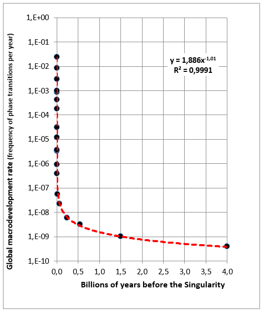
Fig. 17. Scatterplot of the phase transition points from Panov’s list with the fitted power-law regression line (with a logarithmic scale for the Y-axis) – for the Singularity date identified as 2027 CE with the least squares method

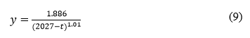
In the double logarithmic scale the fit between the power-lower model
y = 1,886/x^1,01 (where x denotes number of years before the singularity point defined as 2027 CE) and the empirical estimates of Panov looks as follows (see Fig. 18).

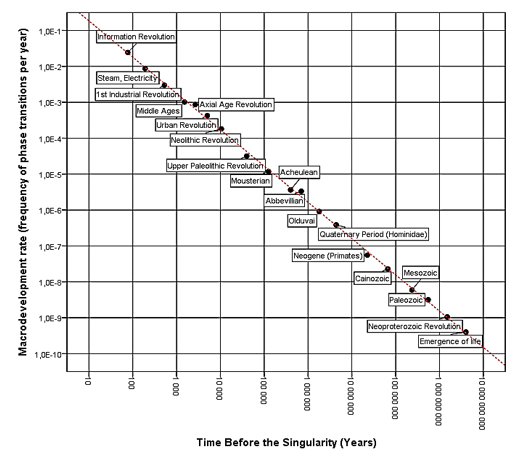
Fig. 18. Scatterplot of the phase transition points from Panov’s list with the fitted power-law regression line (double logarithmic scale) – for the Singularity date identified as 2027 CE with the least squares method

Actually, I expected that the equation best describing the Panov series should look fairly similar to the one best describing the Modis – Kurzweil one; but, to tell the truth, I did not expect that they would look SO SIMILAR (especially, keeping in mind that Modis and Panov relied on totally different sources, and that the resultant lists of ‘canonical milestones’ were very far from being identical).

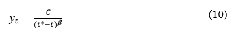
However, the resultant equations turned out to be EXTREMELY similar (this is especially striking taking into consideration the point that neither Modis, nor Panov tried to approximate their time series with Eq. (10)). Indeed, in the unsimplified form the power-law equation best describing the acceleration pattern in the Modis – Kurzweil series looks as follows (see Fig. 10 above):

where, let us recollect, y is the global macrodevelopment rate (number of phase transitions per a unit of time), and 2029 CE is the best-fit singularity point estimate.

In the meantime, the power-law equation best describing the acceleration pattern in the Panov (2005a) series looks as follows (see Fig. 18 above):

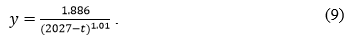
In general form, the respective equation looks as follows:

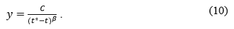
This equation has three parameters – C, t*, and β. Note that all the three parameters turn out to be extremely close for both Modis – Kurzweil and Panov.

Formulas of the Acceleration
of Global Macroevolutionary Development in Panov
and Modis – Kurzweil Series: A Comparison

Indeed, the comparison of the best-fit power-law equations for both series yields the following results (see Table 3):

Table 3. Comparison between two acceleration formulas

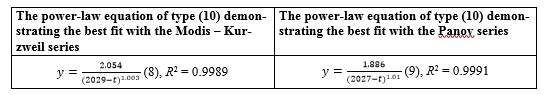
Actually, for me the most impressive result was not even that the singularity (t*) parameters for both regressions have turned out to be so close (just
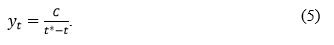
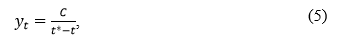
2-year difference!) but that exponent β in both cases has turned out to be so close to 1, which, incidentally, allows to reduce an already very simple power-law Eq. (10)

to an even simpler hyperbolic Eq. (5):

Even the third parameter in Eq. (10) also turns out to be very similar for both Modis – Kurzweil (C = 2.1) and Panov (C = 1.9).

A special remark should be said about the extremely close fit that theoretical curves generated by the extremely simple equations of (5) type demonstrate with both Modis – Kurzweil and Panov series. With respect to Modis – Kurzweil Eq. (5) describes 99,89 % of all the variation of planetary macroevolution development rate in the period of a few billion of years, whereas for Panov this fit reaches whopping 99,91 % – on the other hand, the extreme closeness of R² values for both regressions (just a 0.02 % difference!) is rather impressive in itself (I would stress again that it looks especially impressive taking into consideration the fact that neither Modis, nor Panov tried to approximate their time series with equations (5) or (10)).

Needless to say, that the differential acceleration pattern for Panov also turns out to be very close to Modis – Kurzweil.

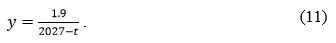
Indeed, as we have already mentioned, there are sufficient grounds to simplify Eq. (9)

to the simple hyperbolic version (11):

As we remember, such an algebraic equation can be regarded as a solution of the following differential equation that is very similar to the one that we obtained above for the Modis – Kurzweil series:

Thus, the overall pattern of acceleration of planetary macroevolution that describes so accurately the Panov series of ‘biospheric revolutions’ turns out to be virtually identical with the one that we have detected above for the Modis – Kurzweil series: ‘the increase in macroevolutionary development rate a times is accompanied by a² increase in the acceleration speed of this development rate; thus, a twofold increase in macroevolutionary development rate n times tends to be accompanied by a fourfold increase in the acceleration speed of this development rate; an increase in macroevolutionary development rate 10 times tended to be accompanied by 100 times increase in the acceleration speed of this development rate; and so on…’.

To my mind, all these indicate the existence of sufficiently rigorous global macroevolutionary regularities (describing the evolution of complexity on our planet for a few billion of years), which can be surprisingly accurately described by extremely simple mathematical functions.

A Striking Discovery of Heinz von Foerster

It appears appropriate to recollect at this point that in their famous article published in the journal Science in 1960 von Foerster, Mora, and Amiot presented their results of the analysis of the world population growth pattern. They showed that between 1 and 1958 CE the world's population (N) dynamics can be described in an extremely accurate way with the following astonishingly simple equation:

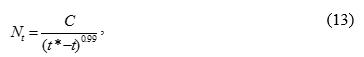
where N_t is the world population at time t, and C and t* are constants, with t* corresponding to the so called ‘demographic singularity’. Parameter t* was estimated by von Foerster and his colleagues as 2026.87, which corresponds to November 13, 2026; this made it possible for them to supply their article with a public-relations masterpiece title – ‘Doomsday: Friday, 13 November, A.D. 2026’ (von Foerster, Mora, and Amiot 1960). Note that von Foerster and his colleagues detected the hyperbolic pattern of world population growth for 1 CE –1958 CE; later it was shown that this pattern continued for a few years after 1958, and also that it can be traced for many millennia BCE (Kapitza 1996a, 1996b, 1999; Kremer 1993; Tsirel 2004; Podlazov 2000, 2001, 2002; Korotayev, Malkov, and Khaltourina 2006a, 2006b; Korotayev and Grinin 2013). In fact Kremer (1993) claims that this pattern is traced since 1 000 000 BP, whereas Kapitza (1996a, 1996b, 2003, 2006, 2010) even insists that it can be found since 4 000 000 BP.

It is difficult not to see that the world population growth acceleration pattern detected by von Foerster in the empirical data on the world population dynamics between 1 and 1958 turns out to be virtually identical with the one that has been detected above with respect to both Modis – Kurzweil and Panov series describing the planetary macroevolutionary development acceleration. Note that the power-law regression has yielded for all the three series the value of exponent β being extremely close to 1 (1.003 for the Modis – Kurzweil series, 1.01 for Panov, and 0.99 for von Foerster).

However, the resultant proximity of parameter t* (that is just the singularity time point) estimates is also really impressive (the power-law regression suggests 2029 for the Modis – Kurzweil series, 2027 for Panov series, and just the same 2027 for von Foerster series).^[28]

We have already mentioned that, as was the case with equations (8) and (9) above, in von Foerster's Eq. (13) the denominator's exponent (0.99) turns out to be only negligibly different from 1, and as was already suggested by von Hoerner (1975) and Kapitza (1992, 1999), it can be written more succinctly as

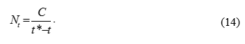
As we see, the resultant equation turns out to be entirely identical with Eq. (5) above that described so accurately the overall planetary macrodevelopment acceleration pattern since at least 4 billion years ago. Note that Eq. (14) has turned out to be as capable to describe in an extremely accurate way the world population dynamics (up to the early 1970s), as Eq. (5) is capable to describe the overall pattern of macrodevelopment acceleration (at least between 4 billion BCE and the present). We will show just an example of such a fit.

Let us take Eq. (14). Now replace t* with 2027 (that is the result of just rounding of von Foester's number, 2026.87), and replace C with 215000.^[29] This gives us a version of von Foerster – von Hoerner – Kapitza Eq. (14) with certain parameters:

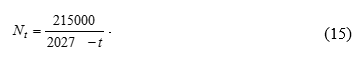
The overall correlation between the curve generated by von Foerster's equation and the most detailed series of empirical estimates looks as follows (see Fig. 19):

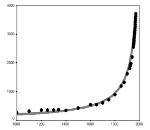
Fig. 19. Correlation between Empirical Estimates of World Population (in millions, 1000 – 1970) and the Curve Generated by von Foerster's Equation (15). Note: black markers correspond to empirical estimates of the world population by McEvedy and Jones (1978) for 1000 – 1950 and UN Population Division (2019) for 1950–1970. The grey curve has been generated by von Foerster's Eq. (15). R² = 0.996

As we see, indeed, Eq. (14) has turned out to be as capable to describe in an extremely accurate way the world population dynamics (up to the early 1970s), as Eq. (5) is capable to describe the overall pattern of global macrodevelopment acceleration.

In the Big History context, it is definitely of great significance that Eq. (5) describing the global acceleration of the macroevolutionary development rates and Eq. (14) describing the world population growth are entirely identical. What is more, both empirical and mathematical analyses indicate that there is a rather deep substantial connection between those two equations, that they describe two different aspects of the same global macroevolutionary process (see Appendix 1 below).

On the Formula of Acceleration
of the Global Evolutionary Development

I must say that I had serious doubts when I first got across calculations of Panov and Modis (and I am not surprised that most historians get very similar doubts when they see their works). I have lots of complaints regarding the accuracy of many of their descriptions of their ‘canonical milestones’, their selection, and their datings (see, e.g., Korotayev 2015). I have only started taking their calculations seriously, when I analyzed myself the two respective time series compiled (as we have seen above) entirely independently by two independently working scientists using entirely different sources with a mathematical model not applied to their analysis either by Modis or by Panov, and found out that they are described in an extremely accurate way by an almost identical mathematical hyperbolic function – suggesting the actual presence of a rather simple hyperbolic planetary macroevolution acceleration pattern observed on the Earth for the last 4 billion years. This impression became even stronger when the equation describing the planetary macroevolution acceleration pattern turned out to be identical with the equation that was found by Heinz von Foerster in 1960 to describe in an extremely accurate way the global population growth acceleration pattern between 1 and 1958 CE.

I had some grounds to expect that the planetary macroevolutionary acceleration in the last 4 billion years could be described by a single hyperbolic equation quite accurately, because our earlier research found that both biological and social macroevolution could be described by rather similar simple hyperbolic equations (Korotayev 2005, 2006a, 2006b, 2007a, 2007b, 2008, 2009, 2012, 2013; Korotayev and Khaltourina 2006; Khaltourina et al. 2006; Korotayev, Malkov, and Khaltourina 2006a, 2006b; Markov and Korotayev 2007, 2008, 2009; Grinin and Korotayev 2009; Markov, Anisimov, and Korotayev 2010; Korotayev and Malkov 2012; Korotayev and Markov 2014, 2015; Grinin, Markov, and Korotayev 2013, 2014, 2015; Korotayev and Malkov 2016; Zin-
kina, Shulgin, and Korotayev 2016; Korotayev, Zinkina, and Andreev 2016; Korotayev and Zinkina 2017), but I must say that even I was really astonished to find such a close fit.

To my mind, all these indicate the existence of sufficiently rigorous global macroevolutionary regularities (describing the evolution of complexity on our planet for a few billions of years), which can be surprisingly accurately described by extremely simple mathematical functions, as well as the presence of a global planetary macroevolutionary development acceleration pattern described by a very simple equation:

where C₁ is a parameter in the following hyperbolic equation:

where t* is the singularity date.

It is also not without interest that the singularity dates in all the three (rather different) cases under consideration have turned out to be almost entirely identical (2029 CE for Modis – Kurzweil, and 2027 CE for both Panov and von Foerster).

Toward the Singularity Interpretation.
The Place of the Singularity in the Big History
and Global Evolution

But how seriously should we take the prediction of ‘singularity’ contained in such mathematical models? Should we really expect with Kurzweil that around 2029 we should deal with a few orders of magnitude acceleration of the tech-nological growth (indeed, predicted by Eq. (4) if we take it literally)?^[30]

I do not think so. This is suggested, for example, by the empirical data on the world population dynamics. As we remember, the global population growth acceleration pattern discovered by Heinz von Foerster is identical with planetary macroevolutionary acceleration patterns of Modis – Kurzweil and Panov, and it is characterized by the singularity parameter (2027 CE) that is simply identical for Panov and has just two-year difference with Modis – Kurzweil. However, what are the grounds to expect that by Friday, November 13, A.D. 2026 the world population growth rate will increase by a few orders of magnitude as is implied by von Foerster equation? The answer to this question is very clear. There are no grounds to expect this at all. Indeed, as we showed quite time ago,

von Foerster and his colleagues did not imply that the world population on that day [November 13, A.D. 2026] could actually become infinite. The real implication was that the world population growth pattern that was followed for many centuries prior to 1960 was about to come to an end and be transformed into a radically different pattern. Note that this prediction began to be fulfilled only in a few years after the ‘Doomsday’ paper was published (Korotayev 2008: 154).

Indeed, starting from the early 1970s the world population growth curve began to diverge more and more from the almost ideal hyperbolic shape it had before (see Figs. 19 and 20) (see, e.g., Kapitza 2003, 2006, 2007, 2010; Livi-Bacci 2012; Korotayev, Malkov, and Khaltourina 2006a, 2006b; Korotayev, Goldstone, and Zinkina 2015; Grinin and Korotayev 2015; UN Population Division 2025), and in recent decades it has been taken more and more clearly logistic shape – the trend towards hyperbolic acceleration has been clearly replaced with the logistic slow-down (see Fig. 20).

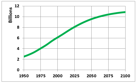
Fig. 20. World population dynamics (billions), empirical estimates of the UN Population Division for 1950–2015 with its middle forecast till 2100

Source: UN Population Division 2019.

In some respect, it may be said that von Foerster did discover the singularity of the human demographic history; it may be said that he detected that the human World System was approaching the singular period in its history when the hyperbolic accelerating trend that it had been following for a few millennia (and even a few millions of years according to some) would be replaced with an opposite decelerating trend. The process of this trend reversal has been studied very thoroughly by now (see, e.g., Vishnevsky 1976, 2005; Chesnais 1992; Caldwell et al. 2006; Khaltourina et al. 2006; Korotayev, Malkov, and Khaltourina 2006a, 2006b; Korotayev 2009; Gould 2009; Dyson 2010; Reher 2011; Livi-Bacci 2012; Choi 2016; Podlazov 2017) and is known as the ‘global demographic transition’ (Kapitza 1999, 2003, 2006, 2010; Podlazov 2017). Note that in case of global demographic evolution the transition from the hyperbolic acceleration to logistic deceleration started a few decades before the singularity point mathematically detected by von Foerster.

There are all grounds to maintain that the deceleration of planetary macroevolutionary development has also already begun – and it started a few decades before the singularity time points detected both in Modis – Kurzweil and Panov.

So, how seriously should we take the prediction of ‘singularity’ contained in hyperbolic mathematical models? For example, could we really use the point that our analysis of the Modis – Kurzweil time series reveals a singularity around 2029 CE as an indication to expect that around this time the transition to Big History Threshold 9 could actually start?

Note that some big historians take such ‘mathematically grounded’ predictions rather seriously. The most prominent among them is Akop Nazaretyan. In his article with a symptomatic title ‘Megahistory and Its Mysterious Singularity’ in the Russian Academy of Sciences flagship journal he maintains the following:

The solar system formed about 4.6 billion years ago, and the very first signs of life on Earth date back to 4 billion years. Thus, our planet became one of the (most likely, numerous) points on which the subsequent evolution of the metagalaxy was localized. Although its acceleration was noted long ago, a new circumstance has been discovered of late. The Australian economist and global historian G. D. Snooks, the Russian physicist A. D. Panov, and the American mathematician R. Kurzweil compared independently, proceeding from different sources and using different mathematical apparatuses, the time intervals between global phase transitions in biological, presocial, and social evolutions (Panov 2005a, 2008; Kurzweil 2005; Snooks 1996; Weinberg 1977). Calculations show that these periods decreased according to a strictly decreasing geometrical progression; in other words, the acceleration of evolution on the Earth followed a logarithmic law (Nazaretyan 2015a: 356).

Furthermore, in his article in the Journal of Globalization Studies he goes on to claim that

having extrapolated the hyperbolic curve into the future, the researchers have come to a nearly unanimous (ignoring the individual interpretations) and even more striking result: around the mid-21^st century, the hyperbole turns into a vertical. That is, the speed of the evolutionary processes tends to infinity, and the time intervals between new phase transitions vanish (Nazaretyan 2017: 32; see also Nazaretyan 2015a: 357).

As we see, Nazaretyan does use the mathematical calculations of the singularity point for the global evolutionary hyperbola to predict the possible timing of Threshold 9 (that according to him should be much more profound than preceding Thresholds 7 (‘Agricultural Revolution’) and 8 (‘Modern Revolution’).

However, do the calculations presented by Panov in 2003–2005, or by us above, really give grounds to expect ‘the Singularity’/onset of Big History Threshold 9 between 2029 and 2050 CE? I do not think so.

In fact, as we can see, our paper appears to be the first attempt to ‘extrapolate the line of the hyperbolic acceleration to the future’.^[31] Contra Nazaretyan, such an attempt was not undertaken by Donald Snooks (1996), who did not try to calculate any mathematical singularities. No formal attempts to ‘extrapolate the line of the hyperbolic acceleration to the future’ using any mathematical techniques have been undertaken by Ray Kurzweil – at least because he seems to be still sure that he is dealing with exponential (but not hyperbolic) acceleration. Thus, almost the only person who (before us) has conducted any attempts to calculate mathematically the singularity time for the line of the acceleration of the planetary evolution appears to be Alexander Panov (2005a, 2005b; see also Panov 2020: Ch. 20) – though in some respects this can be also said about Sergey Grinchenko (see 2001, 2004, 2006a, 2006b, etc., Grinchenko and Shchapova 2020), Theodore Modis (2002, 2003), and David LePoire (2013, 2015, LePoire 2020).

Panov's technique was somehow different from the ‘extrapolation of the line of the hyperbolic acceleration to the future’ (this was rather the technique applied by us), but, no doubt, Panov has applied a rather rigorous mathematical technique to identify the Singularity of the planetary evolution. But what was the result of these calculations? After Panov applied his mathematical analysis to the time series starting from Phase Transition 0 (Emergence of the life on the Earth, ≈ 4 billion BP) to Phase Transition 19 (‘Crisis and collapse of the Communist Block, information globalization’), he found that the mathematical singularity point for this time series is in no way situated somewhere ‘around the mid-21^st century’ as is claimed by Nazaretyan, but in 2004 CE^[32] (Panov 2005a: 130; 2005b: 222). Nazaretyan has even happened to miss that soon after detecting this singularity point, Panov got involved in the study of the processes of the slow-down of the global technological-scientific growth (Panov 2009, 2013; 2020: Ch. 20).

As LePoire puts it, Big History trends of accelerating change and complexity with related increases in energy use may not be sustainable. The indications of potential slowdown in the rate of change in economies, technology, and social response were investigated. This is not to say that change will stop, just the rate of change will not accelerate. In fact, at the inflection point in a logistic learning curve only half of the discoveries have been made. Since there were three major phases in life, human, and technological civilization,^[33] the continuation of the logistic curve would suggest three more phases.^[34] The direction of the development of technologies points to the next phase including enhanced human technology through advanced biotech and computer integration… A rapid change is not necessarily good. It tends to push systems away from efficiency because there are little long-term expectations… (LePoire 2013: 115–116; for more details see LePoire 2020).

As major factors of the starting deceleration LePoire names ‘higher costs of energy and limited natural resources, the diminished rate of fundamental discovery in physical sciences, and the need for investment in environmental maintenance’ (LePoire 2013: 109).

Note that Modis (2002, 2003, 2005, 2012, 2020: Ch. 4) also interprets the maximum acceleration of the complexity growth rate that he detects around 2000 CE as an inflexion point after which we will deal with the deceleration of the global complexity growth rate. In fact, the earliest known to me attempt to detect mathematically a singularity in a series of what Modis would call ‘canonical milestones’ of planetary evolution^[35] was undertaken in 2001 (thus, just a year before Modis' seminal article in Technological Forecasting and Social Change) by Sergey Grinchenko (2001, 2004, 2006a, 2006b, 2007, 2011, 2015; Grinchenko and Shchapova 2010, 2016, 2017a, 2017b; 2020: Ch. 10; Shchapova and Grinchenko 2017); the singularity point was detected by him mathematically^[36] as 1981 CE, whereas the subsequent period was interpreted by Grinchenko as a period of deceleration of the ‘metaevolution rate’. Note that this correlates very well with our detection of 1973 CE as an inflection point, after which the hyperbolic acceleration of the world population growth (as well as the quadratic hyperbolic acceleration of the world GDP growth) started to be replaced in the long term by the opposite deceleration trend (Korotayev 2006a; Korotayev et al. 2010; Korotayev and Bogevolnov 2010; Akaev et al. 2014; Sadovnichy et al. 2014; Korotayev and Bilyuga 2016). This is well supported by the growing body of evidence suggesting the start of the long term deceleration of the global techno-scientific and economic growth rates in the recent decades (see, e.g., Krylov 1999, 2002, 2007; Huebner 2005; Khaltourina and Korotayev 2007; Maddison 2007; Korotayev and Bogevolnov 2010; Korotayev et al. 2010; Modis 2002, 2005, 2012; Akaev 2010; Gordon 2012; Teulings and Baldwin 2014; Piketty 2014; LePoire 2005, 2009, 2013, 2015; Korotayev and Bilyuga 2016; Popović 2018, etc.; see also Modis 2020: Ch. 4; LePoire and Chandrankunnel 2020: Ch. 9; LePoire and Devezas 2020: Ch. 11; Widdowson 2020: Ch. 22).

Conclusion

Thus, the analysis above appears to indicate the existence of sufficiently rigorous global macroevolutionary regularities (describing the evolution of complexity on our planet for a few billion years), which can be surprisingly accurately described by extremely simple mathematical functions. At the same time this analysis suggests that in the region of the singularity point there is no reason, after Kurzweil, to expect an unprecedented (many orders of magnitude) acceleration of the rates of technological development. There are more grounds for interpreting this point as an indication of an inflection point, after which the pace of global evolution will begin to slow down systematically in the long term.

References

A. H. 1975. Mesozoic Era. The New Encyclopedia Britanica, 15^th ed., Vol. 11. Encyclopedia Britanica, pp. 1013–1017. Chicago, IL.

A. P. 1975. Cenozoic Era. The New Encyclopedia Britanica, 15^th ed., Vol. 3. Encyclopedia Britanica, pp. 1079–1083. Chicago, IL.

Adams H. 1969 [1909]. The Rule of Phase Applied to History. The Degradation of the Democratic Dogma / Ed. by H. Adams, pp. 267–311. New York, NY: Harper & Row.

Akaev A. 2010. Fundamental Limits to Economic Growth and Consumption. System Monitoring of Global and Regional Risks 2: 12–30. In Russian (Акаев А. Фундаментальные пределы экономического роста и потребления. Системный мониторинг глобальных и региональных рисков 2: 12–30).

Akaev A, Korotayev A, and Malkov S (Eds.) 2014. Current Situation and Contours of the Future. Complex System Analysis, Mathematical Modeling and Forecasting of Development of BRICS Countries. Preliminary Results / Ed. by A. A. Akaev, A. V. Korotayev, and S. Yu. Malkov, pp. 10–31. Moscow: Krasand/URSS. In Russian (Ака-
ев А., Коротаев А. В., Малков С. Ю. Современная ситуация и контуры будущего. Комплексный системный анализ, математическое моделирование и про-
гнозирование развития стран БРИКС. Предварительные результаты, с. 10–31. М.: Красанд/УРСС).

Alvarez L. W., Alvarez W., Asaro F., and Michel H. V. 1980. Extraterrestrial Cause for the Cretaceous-Tertiary Extinction. Science 208(4448): 1095–1108. https://doi.
org/10.1126/science.208.4448.1095

Antiseri D., and Reale G. 2001. Western Philosophy from Its Origins to the Present Day. Antiquity, the Middle Ages. Saint Petersburg: Petropolis. In Russian (Антисе-
ри Д., Реале Дж. Западная философия от истоков до наших дней. Антич-ность, Средние века. Санкт-Петербург: Петрополис).

Baker D. 2014. Standing on the Shoulders of Giants: Collective Learning as a Key Concept in Big History. Teaching & Researching Big History: Exploring a New Scholarly Field / Ed. by L. Grinin, D. Baker, E. Quaedackers, and A. Korotayev,
pp. 41–64. Volgograd: ‘Uchitel’.

Baker D. 2015a. Collective Learning: A Potential Unifying Theme of Human History. Journal of World History 26(1):77–104. https://doi.org/10.1353/jwh.2016.0006

Baker D. 2015b. Standing on the Shoulders of Giants: Collective Learning as a Key Concept in Big History. Globalistics and Globalization Studies 4: 301–318.

Barrow J. D., and Silk J. 1980. The Structure of the Early Universe. Scientific American 242(4): 118–128.

Begun D. R. 2003. Planet of the Apes. Scientific American 289(2): 64–73.

Begun D. R. 2004. Planet of the Anthropoids. V mire nauki (11): 68–77.

Boriskovsky P. 1970. Acheulean Culture. Great Soviet Encyclopedia Vol. 2, p. 471. Moscow: Sovetskaya entsiklopediya In Russian (Борисковский П. Ашельская культура. Большая советская энциклопедия. Т. 2., с. 471. М.: Советская энциклопедия).

Boriskovsky P. 1974a. Oldovay. Great Soviet Encyclopedia. Vol. 18, p. 369. Moscow: Sovetskaya entsiklopediya. In Russian (Борисковский П. Олдовай. Большая советская энциклопедия. Т. 18, с. 369. М.: Советская энциклопедия).

Boriskovsky P. 1974b. The Mousterian. Great Soviet Encyclopedia . Vol. 17, p. 134. M.: Sovetskaya entsiklopediya. In Russian (Борисковский П. Мустьерская культура. Большая советская энциклопедия. Т. 17, с. 134. М.: Советская энциклопедия).

Boriskovsky P. 1978. Сhellean Culture. Great Soviet Encyclopedia Vol. 29, p. 377. Moscow: Sovetskaya entsiklopediya In Russian (Борисковский П. Шелльская культура. Большая советская энциклопедия. Т. 29, с. 377. М.: Советская энциклопедия).

Burenhult G. (Ed.) 1993. The First Humans: Human Origins and History to 10,000 BC. Harper, San Francisco, CA.

Caldwell J. C., Caldwell B. K., Caldwell P., McDonald P. F., and Schindlmayr T. 2006. Demographic Transition Theory. Dordrecht: Springer. https://doi.org/10.1007/
978-1-4020-4498-4

Callaghan V., Miller J., Yampolskiy R., and Armstrong S. 2017. Technological Singularity. Dordrecht: Springer. https://doi.org/10.1007/978-3-662-54033-6

Carrol R. L. 1988. Vertebrate Paleontology and Evolution. New York, NY: W.H. Freeman and Company.

Carrol R. L. 1992. Paleontology and Evolution of Vertebrates. Vol. 1. Moscow: Mir. In Russian (Кэролл Р. Палеонтология и эволюция позвоночных. Т. 1. М.: Мир).

Carrol R. L. 1993a. Paleontology and Evolution of Vertebrates. Vol. 2. Moscow: Mir. In Russian (Кэролл Р. Палеонтология и эволюция позвоночных. Т. 2. М.: Мир).

Carrol R. L. 1993b. Paleontology and Evolution of Vertebrates. Vol. 3. Moscow: Mir. In Russian (Кэролл Р. Палеонтология и эволюция позвоночных. Т. 3. М.: Мир).

Chesnais J. C. 1992. The Demographic Transition: Stages, Patterns, and Economic Implications. Oxford: Clarendon Press.

Choi Y. 2016. Demographic Transition in Sub-Saharan Africa: Implications for Demographic Dividend. Demographic Dividends: Emerging Challenges and Policy Implications / Ed. by R. Pace, and R. Ham-Chande, pp. 61–82. Dordrecht: Springer. https://doi.org/10.1007/978-3-319-32709-9_4

Christian D. 2005. Maps of Time: An Introduction to Big History. Berkeley, CA: University of California Press.

Christian D. 2014. Swimming Upstream: Universal Darwinism and Human History. Teaching & Researching Big History: Exploring a New Scholarly Field / Ed. by
L. Grinin, D. Baker, E. Quaedackers, and A. Korotayev, pp. 19–40. Volgograd: Uchitel.

Christian D. 2015. Swimming Upstream: Universal Darwinism and Human History. Globalistics and Globalization Studies 4: 138–154.

Diakonov I. 1994. The Paths of History. From Ancient Man to the Present Day. Moscow: Vostochnaya literatura. In Russian (Дьяконов И. Пути истории. От древнейшего человека до наших дней. М.: Восточная литература).

Diakonov I. 1999. The Paths of History. Cambridge: Cambridge University Press.

Dyson T. 2010. Population and Development. The Demographic Transition. London: Zed Books.

Eden A. H., Moor J. H., Søraker J. H., and Steinhart E. (Eds.) 2012. Singularity Hypotheses: A Scientific and Philosophical Assessment. Berlin: Springer. https://
doi.org/10.1007/978-3-642-32560-1

Fedonkin М. 2003. Narrowing of Life Geochemical Basis and Biosphere Eukaryotization: Causal Links. Paleontologicheskiy zhurnal (6): 33–53. In Russian (Федонкин М. Сужение геохимического базиса жизни и эукариотизация биосферы: причинная связь. Палеонтологический журнал (6): 33–53).

von Foerster H., Mora P. M., and Amiot L. W. 1960. Doomsday: Friday, 13 November, AD 2026. Science 132(3436): 1291–1295. https://doi.org/10.1126/science.132.
3436.1291

Foley R. 1990. Another Unique Species. Ecological Aspects of Human Evolution. Moscow: Mir. In Russian (Фоули Р. Еще один неповторимый вид. Экологические аспекты эволюции человека Moscow: Mir).

Fomin A. 2020. Hyperbolic Evolution from Biosphere to Technosphere. The 21st Century Singularity and Global Futures. A Big History Perspective / Ed. by A. Korotayev, and D. LePoire, pp 86–96. Cham: Springer.

Galimov E. 2001. The Phenomenon of Life: Between Equilibrium and Nonlinearity. Origin and Principles of Evolution. Moscow: URSS. In Russian (Галимов Э. Феномен жизни. Между равновесием и нелинейностью. Происхождение и принципы эволюции. М.: УРСС).

Gordon R. J. 2012. Is US Economic Growth over? Faltering Innovation Confronts the Six Headwinds. Cambridge, MA: National Bureau of Economic Research.

Gould W. T. S. 2009. Population and Development. London: Routledge.

Grinchenko S. 2001. Social Metaevolution of Humanity as a Sequence of Steps in the Formation of Mechanisms of Its Systemic Memory. Issledovano v Rossii 145: 1652–1681. In Russian (Гринченко С. Социальная метаэволюция Человечества как последовательность шагов формирования механизмов его системной памяти. Исследовано в России 145: 1652–1681).

Grinchenko S. 2004. Systemic Memory of a Living Being (as the Basis of Its Metaevolution and Periodic Structure). Moscow: Mir. In Russian (Гринченко С. Системная память живого (как основа его метаэволюции и периодической структуры). М.: Мир).

Grinchenko S. 2006a. Meta-evolution of Nature System – The Framework of History. Social Evolution & History 5(1): 42–88.

Grinchenko S. 2006b. The History of Mankind from the Information and Cybernetic Positions. History and Mathematics: Problems of Periodization of Historical Macroprocesses / Ed. by S. P. Kapitsa et al., pp. 38–52. In Russian (Гринченко С. История человечества с информатико-кибернетических позиций. История
и математика: проблемы периодизации исторических макропроцессов / Ред.
С. П. Капица и др., с. 38–52).

Grinchenko S. 2007. Metaevolution (of the System of Inanimate, Animate and Socio-Technological Nature). Moscow: IPI RAN. In Russian (Гринченко С. Метаэволюция (систем неживой, живой и социально-технологической природы). М.: ИПИ РАН).

Grinchenko S. 2011. The Pre- and Post-History of Humankind: What is It? Problems of Contemporary World Futurology / Ed. by V. I. Yakunin, pp. 341–353. Newcastle-upon-Tyne: Cambridge Scholars Publishing.

Grinchenko S. 2015. Modeling: Industrial and Deductive. Problems of Historical Knowledge / Ed. by K. Khvostova, pp. 95–101. Moscow: IVI RAN. In Russian (Гринченко С. Моделирование: индуктивное и дедуктивное. Проблемы исторического познания / Ред. К. Хвостова, с. 95–101. М.: ИВИ РАН).

Grinchenko S., and Shchapova Yu. 2010. Human History Periodization Models. Herald of the Russian Academy of Sciences 80(6): 498–506. https://doi.org/10.1134/
S1019331610060055

Grinchenko S., and Shchapova Yu. 2016. Archaeological Epoch as the Succession of Generations of Evolutive Subject-Carrier Archaeological Sub-Epoch. Philosophy of Nature in Cross-Cultural Dimensions. The Result of the International Symposium at the University of Vienna. Komparative Philosophie und Interdisziplinäre Bildung, pp. 423–439. Vienna: University of Vienna.

Grinchenko S., and Shchapova Yu. 2017a. Archaeological Epoch as the Succession of Generations of Evolutive Subject-Carrier Archaeological Sub-Epoch. Philosophy of Nature in Cross-Cultural Dimensions, pp. 478–499. Hamburg: Verlag Dr. Kovač.

Grinchenko S., and Shchapova Yu. 2017b. Paleoanthropology, Chronology and Periodization of the Archaeological Epoch: A Numerical Model. Prostranstvo i Vremya 1(27): 72–82. In Russian (Гринченко С., Щапова Ю. Палеоантропология, хронология и периодизация археологической эпохи: числовая модель. Пространство и время 1(27): 72–82.

Grinchenko S., and Shchapova Yu. 2020. The Deductive Approach to Big History's Singularity. The 21st Century Singularity and Global Futures. A Big History Perspective / Ed. by A. Korotayev, and D. LePoire, pp. 169–176. Cham: Springer.

Grinin L. 2006. Periodization of History: A Theoretic-Mathematical Analysis. History & Mathematics: Historical Dynamics and Development of Complex Societies / Ed. by P. Turchin, L. Grinin, V. de Munck, and A. Korotayev, pp. 10–38. Moscow: URSS.

Grinin L., Grinin A., and Korotayev A. 2020. Dynamics of Technological Growth Rate and the 21^st Century Singularity. The 21st Century Singularity and Global Futures. A Big History Perspective / Ed. by A. Korotayev, and D. LePoire, pp. 287–344. Cham: Springer.

Grinin L., and Korotayev A. 2009. Social Macroevolution: Growth of the World System Integrity and a System of Phase Transitions. World Futures 65(7): 477–506. https://doi.org/10.1080/02604020902733348

Grinin L., and Korotayev A. 2015. Great Divergence and Great Convergence. A Global Perspective. Cham: Springer. https://doi.org/10.1007/978-3-319-17780-9

Grinin L., Markov A., and Korotayev A. 2013. On Similarities between Biological and Social Evolutionary Mechanisms: Mathematical Modeling. Cliodynamics 4(2): 185–228. https://doi.org/10.21237/C7clio4221334

Grinin L., Markov A., and Korotayev A. 2014. Mathematical Modeling of Biological and Social Evolutionary Macrotrends. History & Mathematics: Trends and Cycle / Ed. by L. Grinin, and A. Korotayev, pp. 9–48. Volgograd: Uchitel.

Grinin L., Markov A., and Korotayev A. 2015. Modeling of Biological and Social Phases of Big History. Evolution: From Big Bang to Nanorobots / Ed. by L. Grinin, and A. Korotayev, pp. 111–150. Volgograd: Uchitel.

Heidmann J. 1989. Cosmic Odyssey. Cambridge: Cambridge University Press.

von Hoerner S. J. 1975. Population Explosion and Interstellar Expansion. Journal of the British Interplanetary Society 28: 691–712.

Huebner J. 2005. A Possible Declining Trend for Worldwide Innovation. Technological Forecasting and Social Change 72(8): 980–986. https://doi.org/10.1016/j.tech
fore.2005.01.003

JBW. 1975. Paleozoic Era, Upper. The New Encyclopedia Britannica, 15^th ed., Vol. 13, Encyclopedia Britannica, pp. 921–930. Chicago, IL.

Jaspers K. 1991. The Meaning and Purpose of the History. Moscow: Politizdat. In Russian (Ясперс К. Смысл и назначение истории. М.: Политиздат).

Johanson D., and Edgar B. 1996. From Lucy to Language. New York, NY: Simon and Schuster.

Kapitza S. 1992. Mathematical Model of Global Population Growth. Mathematical Modelling 4(6): 65–79. In Russian (Капица С. Математическая модель роста населения мира. Математическое моделирование 4(6): 65–79).

Kapitza S. 1996a. The Phenomenological Theory of World Population Growth. Physics-uspekhi 39(1): 57–71. https://doi.org/10.1070/PU1996v039n01ABEH000127

Kapitza S. 1996b. The Phenomenological Theory of Human Population Growth. Uspekhi fizicheskikh nauk 166(1): 63–80. In Russian (Капица С. Феноменологическая теория роста населения Земли. Успехи физических наук 166(1): 63–80).

Kapitza S. 1999. How Many People Lived, Live and Will Live on Earth? Moscow: Nauka. In Russian (Капица С. Сколько людей жило, живет и будет жить на земле? М.: Наука).

Kapitza S. 2003. The Statistical Theory of Global Population Growth. Formal Descriptions of Developing Systems / Ed. by J. Nation, I. Trofimova, J. D. Rand, and
W. Sulis, pp. 11–35. Dordrecht: Springer. https://doi.org/10.1007/978-94-010-0064-2_2

Kapitza S. 2006. Global Population Blow-Up and After. Hamburg: Global Marshall Plan Initiative.

Kapitza S. 2007. Demographic Transition and the Future of Humanity. Vestnik Evropy (21): 7–16. In Russian (Капица С. Демографический переход и будущее человечества. Вестник Европы (21): 7–16).

Kapitza S. 2010. On the Theory of Global Population Growth. Physics-Uspekhi 53(12): 1287–1296. https://doi.org/10.3367/UFNe.0180.201012g.1337

Khaltourina D., and Korotayev A. 2007. A Modified Version of a Compact Mathematical Model of the World System Economic, Demographic, and Cultural Development. Mathematical Modeling of Social and Economic Dynamics / Ed. by
M. Dmitriev, A. Petrov, and N. Tretyakov, pp. 274–277. Moscow: RUDN.

Khaltourina D., Korotayev A., and Malkov A. 2006. A Compact Macromodel of the World System Demographic and Economic Growth, 1–1973 CE. Cybernetics and Systems. Vol. 1. Austrian Society for Cybernetic Research / Ed. by R. Trappl,
pp. 330–335. Vienna: Austrian Society for Cybernetic Research.

Keller B. 1975. Paleozoic Group (Era). The Great Soviet Encyclopedia. Vol. 19. Moscow: Sovetskaya entsiklopediya.

Korotayev A. 2005. A Compact Macromodel of World System Evolution. Journal of World-Systems Research 11(1): 79–93. https://doi.org/10.5195/jwsr.2005.401

Korotayev A. 2006a. The World System History Periodization and Mathematical Models of Socio-Historical Processes. History & Mathematics: Analyzing and Modeling Global Development 1: 39–98.

Korotayev A. 2006b. The World System Urbanization Dynamics: A Quantitative Analysis. History & Mathematics: Historical Dynamics and Development of Complex Societies 2: 44–62.

Korotayev A. 2007a. Compact Mathematical Models of World System Development, and How They Can Help Us to Clarify Our Understanding of Globalization Processes. Globalization as Evolutionary Process: Modeling Global Change / Ed. by
G. Modelski, T. Devezas, and W. Thompson, pp. 133–160. London: Routledge.

Korotayev A. 2007b. Secular Cycles and Millennial Trends: A Mathematical Model. Mathematical Modeling of Social and Economic Dynamics / Ed. by M. Dmitriev,
A. Petrov, and N. Tretyakov, pp. 118–125. Moscow: RUDN.

Korotayev A. 2008. Globalization and Mathematical Modeling of Global Development. Hierarchy and Power in the History of Civilizations: Political Aspects of Modernity / Ed. by L. Grinin, D. Beliaev, and A. Korotayev, pp. 225–240. Moscow: LIBROCOM/
URSS.

Korotayev A. 2009. Compact Mathematical Models of the World System Development and Their Applicability to the Development of Local Solutions in Third World Countries. Systemic Development: Local Solutions in a Global Environment / Ed. by J. Sheffield, pp. 103−116. Litchfield Park, AZ: ISCE Publishing.

Korotayev A. 2012. Globalization and Mathematical Modeling of Global Development. Globalistics and Globalization Studies 1: 148–158.

Korotayev A. 2013. Globalization and Mathematical Modeling of Global Evolution. Evolution: Development within Big History, Evolutionary and World-System Paradigms / Ed. by L. Grinin, and A. Korotayev, pp. 69–83. Volgograd: Uchitel.

Korotayev A. 2015. Singular Points of Big History. Archimedes Singularity. Paper presented at the 2^nd International Symposium ‘Big History and Global Evolution’, October 27–29, 2015, Lomonosov Moscow State University. URL: https://www.
academia.edu/39090913/Korotayev_A_2015_Singular_Points_of_Big_History._Archi
medes_Singularity._Paper_presented_at_the_2nd_Symposium_Big_History_and_
Global_Evolution_October_27_29_2015_Moscow_State_University._SHORT_
VERSION

Korotayev A., and Bilyuga S. 2016. On Some Current Trends in Global Economic Development. Vestnik Instituta ekonomiki Rossiyskoy akademii nauk (4): 20–39. In Russian (Коротаев А. В., Билюга С. О некоторых современных тенденциях мирового экономического развития. Вестник института экономики Российской академии наук (4): 20–39).

Korotayev A., and Bogevolnov J. 2010. Some General Trends in the Economic Development of the Global System. Forecasting and Modeling of Crises and Global Dynamics / Ed. by A. Akaev, A. Korotayev, and G. Malinetsky, pp. 161–171. Moscow: LKI/URSS. In Russian (Коротаев А. В., Божевольнов Ю. Некоторые общие тенденции экономического развития Мир-Системы. Прогноз и моделирование кризисов и мировой динамики / Ред. А. Акаев, А. Коротаев, Г. Малинецкий,
с. 161–171. М.: ЛКИ/URSS).

Korotayev A., Goldstone J., and Zinkina J. 2015. Phases of Global Demographic Transition Correlate with Phases of the Great Divergence and Great Convergence. Technological Forecasting and Social Change 95: 163–169. https://doi.org/10.1016/
j.techfore.2015.01.017

Korotayev A., and Grinin L. 2013. Urbanization and Political Development of the World System. Entelequia. Revista interdisciplinar 15: 197–254.

Korotayev A., and Khaltourina D. 2006. Introduction to Social Macrodynamics: Secular Cycles and Millennial Trends in Africa. Moscow: KomKniga/URSS.

Korotayev A., Khaltourina D., Malkov A., Bogevolnov J., Kobzeva S., and Zinkina J. 2010. Laws of History. Mathematical Modeling and Forecasting of World and Regional Development. Moscow: LKI/URSS. In Russian (Коротаев А. В., Халту-рина Д., Малков А., Божевольнов Ю., Кобзева С., Зинькина Ю. Законы истории. Математическое моделирование и прогнозирование мирового и регионального развития. М.: ЛКИ/URSS).

Korotayev A., and Malkov A. 2016. A Compact Mathematical Model of the World System Economic and Demographic Growth, 1 CE – 1973 CE. International Journal of Mathematical Models and Methods in Applied Sciences 10: 200–209.

Korotayev A., Malkov A., and Khaltourina D. 2006a. Introduction to Social Macrodynamics: Compact Macromodels of the World System Growth. Moscow: KomKniga/URSS.

Korotayev A., Malkov A., and Khaltourina D. 2006b. Introduction to Social Macrodynamics: Secular Cycles and Millennial Trends. Moscow: KomKniga/URSS.

Korotayev A., and Malkov S. 2012. Mathematical Models of the World-System Development. Routledge Handbook of World-Systems Analysis / Ed. by S. Babones, and Ch. Chase-Dunn, pp. 158–161. London: Routledge.

Korotayev A., and Markov A. 2014. Mathematical Modeling of Biological and Social Phases of Big History. Teaching & Researching Big History: Exploring a New Scholarly Field / Ed. by L. Grinin, D. Baker, E. Quaedackers, and A. Korotayev,
pp. 188–219. Volgograd: Uchitel.

Korotayev A., and Markov A. 2015. Mathematical Modeling of Biological and Social Phases of Big History. Globalistics and Globalization Studies 4: 319–343.

Korotayev A., and Zinkina J. 2017. Systemic Boundary Issues in the Light of Mathematical Modeling of World-System Evolution. Journal of Globalization Studies 8(1): 78–96.

Korotayev A., Zinkina J., and Andreev A. 2016. Secular Cycles and Millennial Trends. Cliodynamics 7(2): 204–216. https://doi.org/10.21237/C7CLIO7230484

Kremer M. 1993. Population Growth and Technological Change: One Million B.C. to 1990. The Quarterly Journal of Economics 108: 681–716. https://doi.org/10.2307/
2118405

Kring D., and Durda D. D. 2004. The Day the World Was Burned. V mire nauki 3: 56–63. In Russian (Кринг Д., Дурда Д. Д. День, когда мир был сожжен. В мире науки 3: 56–63).

Krylov O. 1999. Will There be an End to Science? Rossiyskiy khimicheskiy zhurnal 43(6): 96–106. In Russian (Крылов О. Будет ли конец науке? Российский химический журнал 43(6): 96–106).

Krylov O. 2002. Dynamics of Development of Chemical Science. Rossiyskiy khimicheskiy zhurnal 46(3): 96–99. In Russian (Крылов О. Динамика развития химической науки. Российский химический журнал 46(3): 96–99).

Krylov O. 2007. Modern Science: Near End or Completion of Another Stage? Rossiyskiy khimicheskiy zhurnal 51(3): 71–78. In Russian (Крылов О. Современная наука: близкий конец или завершение очередного этапа? Российский химический журнал 51(3): 71–78).

Kurzweil R. 2001. The Law of Accelerating Returns. URL: https://www.kurzweilai.net/
the KOROTAYEV_andrey_sing-law-of-accelerating-returns.

Kurzweil R. 2005. The Singularity Is Near: When Humans Transcend Biology. New York, NY: Viking Penguin.

LePoire D. J. 2005. Application of Logistic Analysis to the History of Physics. Technological Forecasting and Social Change 72(4): 471–479. https://doi.org/10.1016/
S0040-1625(03)00044-1

LePoire D. J. 2009. Exploration of Connections between Energy Use and Leadership Transitions. Systemic Transitions: Past, Present, and Future / Ed. by W. Thompson, pp. 205–220. New York, NY: Palgrave Macmillan. https://doi.org/10.1057/9780230
618381_10

LePoire D. J. 2013. Potential Economic and Energy Indicators of Inflection in Complexity. Evolution: Development within Big History, Evolutionary and World-System Paradigms / Ed. by L. Grinin, and A. Korotayev, pp. 108–118.

LePoire D. J. 2015. Interpreting ‘Big History’ as Complex Adaptive System Dynamics with Nested Logistic Transitions in Energy Flow and Organization. Emergence: Complexity and Organization 17(1): 1–5.

LePoire D. J. 2020. Exploring the Singularity Concept within Big History. The 21st Century Singularity and Global Futures. A Big History Perspective. / Ed. by A. Korotayev, and D. LePoire, pp. 77–97. Cham: Springer.

LePoire D. J. and Chandrankunnel M. 2020. Energy Flow Trends in Big History. The 21st Century Singularity and Global Futures. A Big History Perspective / Ed. by
A. Korotayev, and D. LePoire, pp. 185–200. Cham: Springer.

LePoire D. J., and Devezas T. 2020. Near-term Indications and Models of a Singularity Trend. The 21^st Century Singularity and Global Futures. A Big History Perspective / Ed. by A. Korotayev, and D. LePoire, pp. 213–224. Cham: Springer.

Livi-Bacci M. 2012. A Concise History of World Population. Chichester: Wiley-Blackwell.

Lopatin N. 1983. Ancient Biospheres and the Genesis of Fossil Fuels. Paleontology and the Evolution of the Biosphere. Proceedings of the XXV session of the All-Union Paleontological Society. Leningrad: AN SSSR. In Russian (Лопатин Н. Древние биосферы и генезис горючих ископаемых. Палеонтология и эволюция биосферы. Труды XXV сессии Всесоюзного палеонтологического общества).

Maddison A. 2007. Contours of the World Economy, 1–2030. Oxford: Oxford University Press.

Markov A., Anisimov V., and Korotayev A. 2010. Relationship between Genome Size and Organismal Complexity in the Lineage Leading from Prokaryotes to Mammals. Paleontological Journal 44(4): 363–373. https://doi.org/10.1134/S0031030110040015

Markov A., and Korotayev A. 2007. Phanerozoic Marine Biodiversity Follows a Hyperbolic Trend. Palaeoworld 16(4): 311–318. https://doi.org/10.1016/j.palwor.2007.
01.002

Markov A., and Korotayev A. 2008. Hyperbolic Growth of Marine and Continental Biodiversity through the Phanerozoic and Community Evolution. Zhurnal obshchei biologii 69(3): 175–194.

Markov A., and Korotayev A. 2009. Hyperbolic Growth in Wildlife and Society. Moscow: LKI/URSS. In Russian (Марков А., Коротаев А. Гиперболический рост в живой природе и обществе. М.: ЛКИ/URSS).

McEvedy C., and Jones R. 1978. Atlas of World Population History. Facts on File. New York.

Modis T. 2002. Forecasting the Growth of Complexity and Change. Technological Forecasting and Social Change 69(4): 377–404. https://doi.org/10.1016/S0040-1625(01)00172-X

Modis T. 2003. The Limits of Complexity and Change. The Futurist 37(3): 26–32.

Modis T. 2005. Discussion of Huebner Article Comments by Theodore Modis. Technological Forecasting and Social Change 72: 987–988. https://doi.org/10.1016/j.tech
fore.2005.05.003

Modis T. 2012. Why the Singularity Cannot Happen. Singularity Hypothesis: A Scientific and Philosophical Assessment / Ed. by A. H. Eden, J. H. Moor, et al., pp. 311–346. Berlin: Springer. https://doi.org/10.1007/978-3-642-32560-1_16

Modis T. 2020. Forecasting the Growth of Complexity and Change – An Update. The 21^st Century Singularity and Global Futures. A Big History Perspective / Ed. by
A. Korotayev, and D. LePoire, pp. 101–104. Cham: Springer.

Muratov M., and Vahrameev V. 1974. Mesozoic Group (Era). Great Soviet Encyclopedia. Vol. 16, pp. 6–8. Moscow. In Russian (Муратов М., Вахрамеев В. Мезозойская группа (эра). Большая Советская энциклопедия. Т. 16, с. 6–8. М.).

Nazaretyan A. 2003. Power and Wisdom: Toward a History of Social Behavior. Journal of the Theory of Social Behaviour 33(4): 405–425. https://doi.org/10.1046/
j.1468-5914.2003.00224.x

Nazaretyan A. 2004. Civilizational Crises in the Context of Universal History. Moscow. In Russian (Назаретян А. Цивилизационные кризисы в контексте Универсальной истории. М.).

Nazaretyan A. 2005a. Big (Universal) History Paradigm: Versions and Approaches. Social Evolution & History 4(1): 61–86.

Nazaretyan A. 2005b. Does History Know the Subjunctive Mood? (A Mega-Historical Look at Alternative Models). Filosofskiye nauki 2: 7–18. In Russian (Назаретян А. Знает ли история солагательное наклонение? (Мегаисторический взгляд на альтернативные модели). Философские науки 2: 7–18).

Nazaretyan A. 2009. Meaning-Making as a Global Problem of Modern Times: A Synergetic View. Voprosy filosofii 5: 3–19. In Russian (Назаретян А. Смыслообразование как глобальная проблема современности: синергетический взгляд. Вопросы философии 5: 3–19).

Nazaretyan A. 2013. Mid-21^st Century: The Riddle of Singularity. Filosofskiye nauki 9: 15–24. In Russian (Назаретян А. Середина XXI века: загадка сингулярности. Философские науки 9: 15–24).

Nazaretyan A. 2014. ‘National Idea’: Russia in the Global Scenarios of the 20^th Century. Istoricheskaya psikhologiya i sotsiologiya istorii 7(1): 75–91. In Russian (Назаретян А. «Национальная идея»: Россия в глобальных сценариях XXI века. Историческая психология и социология истории 7(1): 75–91).

Nazaretyan A. 2015a. Megahistory and Its Mysterious Singularity. Herald of the Russian Academy of Sciences 85(4): 352–361. URL: https://doi.org/10.1134/S10193316
15040061

Nazaretyan A. 2015b. Nonlinear Future: Megahistory, Synergetics, Cultural Anthropology, and Psychology in Global Forecasting. Moscow: Argamak-Media. In Russian (Назаретян А. Нелинейное будущее. Мегаистория, синергетика, культурная антропология и психология в глобальном прогнозировании. М.: Аргамак-Медиа).

Nazaretyan A. 2016. Non-Linear Futures: The ‘Mysterious Singularity’ in View of Mega-History. Between Past Orthodoxies and the Future of Globalization. Contemporary Philosophical Problems / Ed. by A. N. Chumakov, and W. C. Gay, pp. 171–191. Boston: Brill-Rodopi.

Nazaretyan A. 2017. Mega-History and the Twenty-First Century Singularity Puzzle. Social Evolution & History 16(1): 31–52.

Nazaretyan A. 2018. The Polyfurcation Century: Does the Evolution on Earth Have a Cosmological Relevance? Journal of Big History 2(1): 27–41. http://dx.doi.org/
10.22339/jbh.v2i1.2253

Nazaretyan A. 2020. The 21st Century's ‘Mysterious Singularity’ in the Light of the Big History. The 21st Century Singularity and Global Futures. A Big History Perspective / Ed. by A. Korotayev, and D. LePoire, pp. 345–362. Cham: Springer.

Orgel L. E. 1998. The Origin of Life – How Long did It Take? Origins of Life and Evolution of the Biosphere 28: 91–96.

Panov A. 2004. Self-Similar Attractor of Socio-Biological Evolution on Earth and the Hypothesis of a Self-Consistent Galactic Origin of Life. Byulleten' Nauchno-kul'turnogo tsentra SETI Akademii kosmonavtiki im. K. E. Tsiolkovskogo 7(24): 4–21. In Russian (Панов А. Автомодельный аттрактор социально-биологической эволюции на Земле и гипотеза самосогласованного галактического происхождения жизни. Бюллетень Научно-культурного центра СЭТИ Академии космонавтики им. К. Э. Циолковского 7(24): 4–21).

Panov A. 2005a. Singular Point of History. Obshchestvennyye nauki i sovremennost 1: 122–137. In Russian (Панов А. Сингулярная точка истории. Общественные науки и современность sovremennost 1: 122–137).

Panov A. 2005b. Scaling Law of the Biological Evolution and the Hypothesis of the Self-Consistent Galaxy Origin of Life. Advances in Space Research 36(2): 220–225. https://doi.org/10.1016/j.asr.2005.03.001

Panov A. 2006. Dyakonov Singularity. Istoriya i matematika 1: 31–37. In Russian (Панов А. Сингулярность Дьяконова. История и математика 1: 31–37).

Panov A. 2008. Universal Evolution and the Problem of the Search for Extraterrestrial Intelligence (SETI). Moscow: LKI/URSS. In Russian (Панов А. Универсальная эволюция и проблема поиска внеземного разума (SETI). М.: ЛКИ/УРСС).

Panov A. D. 2009. Science as a Phenomenon of Evolution. Evolution: Cosmic, Biological, and Social / Ed. by L. E. Grinin, A. V. Markov, and A. V. Korotayev, pp. 99–127. Moscow: LIBROKOM/URSS. In Russian (Панов А. Д. Наука как явление эволюции. Эволюция: космическая, биологическая, социальная / Ред. Л. Е. Гринин, А. В. Марков, А. В. Коротаев, с. 99–127. М.: ЛИБРОКОМ/URSS).

Panov A. 2011. Post-singular Evolution and Post-singular Civilizations. Evolution 2: 212–231.

Panov A. 2013. Macroevolution and Science. Science Studies. Russian Academy of Sciences, Institute of Information on Social Sciences, pp. 215–256. Moscow. In Russian (Панов А. Д. Макроэволюция и наука. Науковедческие исследования. Российская академия наук, Институт информации по общественным наукам,
с. 215–256. М.).

Panov A. 2017. Singularity of Evolution and Post-Singular Development. From Big Bang to Galactic Civilizations. A Big History Anthology / Ed. by B. Rodrigue,
L. Grinin, and A. Korotayev, Vol. III. The Ways that Big History Works: Cosmos, Life, Society and our Future, pp. 370–402. Delhi: Primus Books.

Panov A. 2020. Singularity of Evolution & Post-Singular Development in the Big History Perspective. The 21st Century Singularity and Global Futures. A Big History Perspective / Ed. by A. Korotayev, and D. LePoire, pp. 439–465. Cham: Springer.

Piketty T. 2014. Capital in the Twenty-First Century. Cambridge, MA: The Belknap Press of Harvard University Press.

Podlazov A. 2000. Theoretical Demography as a Basis for Mathematical History. Moscow: IPM RAN.

Podlazov A. 2001. The Basic Equation of Theoretical Demography and the Global Demographic Transition Model. Moscow: IPM RAN. In Russian (Подлазов А. Основное уравнение теоретической демографии и модель глобального демографического перехода. М.: ИПМ РАН).

Podlazov A. 2002. Theoretical Demography. Models of Population Growth and Global Demographic Transition. New Synergetics: A Look into the Third Millennium / Ed. by G. Malinetskiy, and S. Kurdyumov, pp. 324–345. In Russian (Подлазов А. Теоретическая демография. Модели роста народонаселения и глобального демографического перехода. Новая синергетика: взгляд в третье тысячелетие / Ред. Г. Малинецкий, С. Курдюмов, с. 324–345. М.: Наука).

Podlazov A. 2017. A Theory of the Global Demographic Process. Herald of the Russian Academy of Sciences 87(3): 256–266. https://doi.org/10.1134/S10193316170
30054

Popović M. 2018. Technological Progress, Globalization, and Secular Stagnation. Journal of Central Banking Theory and Practice 7(1): 59–100. https://doi.org/10.2478/
jcbtp-2018-0004

Ranj B. 2016. Google's Chief Futurist Ray Kurzweil Thinks We Could Start Living Forever by 2029. Business Insider. April 20. URL: http://www.techinsider.io/googles-chief-futurist-thinks-we-could-start-living-forever-by-2029-2016-4.

Reher D. 2011. Economic and Social Implications of the Demographic Transition. Population and Development Review 37: 11–33. https://doi.org/10.1111/j.1728-4457. 2011.00376.x

Rozanov A. 1986. What Happened 600 Million Years Ago. Moscow: Nauka. In Russian (Розанов А. Что произошло 600 миллионов лет назад. М.: Наука).

Rozanov A. 2003. Fossil Bacteria, Sedimentogenesis, and the Early Biospheric Evolution. Paleontologicheskiy zhurnal 6: 41–49. In Russian (Розанов А. Ископаемые бактерии, седиментогенез и ранние стадии эволюции биосферы. Палеонтологический журнал 6: 41–49).

Rozanov A., and Zavarzin G. 1997. Bacterial Paleontology. Vestnik RAN 67(3): 241–245. In Russian (Розанов А., Заварзин Г. Бактериальная палеонтология. Вестник РАН 67(3): 241–245).

Sadovnichy V., Akaev A., Korotayev A., and Malkov S. 2014. Complex Modeling and Forecasting of the Development of the BRICS Countries in the Context of the World Dynamics. Moscow: Nauka. In Russian (Садовничий В., Акаев А., Коротаев А., Малков С. Комплексное моделирование и прогнозирование развития стран БРИКС в контексте мировой динамики. М.: Наука).

Sagan S. 1989. The Dragons of Eden: Speculations on the Evolution of Human Intelligence. New York, NY: Ballantine Books.

Schopf J. W. (Ed.) 1991. Major Events in the History of Life. Boston, MA: Jones and Bartlett Publishers.

Shanahan M. 2015. The Technological Singularity. Cambridge, MA: MIT Press.

Shantser E. 1973. Cenozoic Group (Era). Great Soviet Encyclopedia. Vol. 11. Soviet Encyclopedia. Moscow. In Russian (Шанцер Е. Кайнозойская группа (эпоха). Большая советская энциклопедия. T. 11. Советская энциклопедия. М.).

Shchapova Yu., and Grinchenko S. 2017. Introduction to the Theory of Archaeological Epoch: Numerical Modeling and Logarithmic Scales of Spatio-Temporal Coordinates. Moscow: Moscow State University. In Russian (Щапова Ю., Гринчен-
ко С. Введение в теорию археологической эпохи: числовое моделирование и логарифмические шкалы пространственно-временных координат. М.: МГУ).

Snooks G. D. 1996. The Dynamic Society: Exploring the Sources of Global Change. London: Routledge.

Snooks G. D. 2005. Big History or Big Theory? Uncovering the Laws of Life. Social Evolution & History 4(1): 160–188.

Snooks G. D. 2020. Is Singularity a Scientific Concept, or the Metaphysical Construct of Historicism? Implications for Big History. The 21st Century Singularity and Global Futures. A Big History Perspective / Ed. by A. Korotayev, and D. LePoire, pp. 225–263. Cham: Springer.

T. K. 1975. Paleozoic Era, Lower. The New Encyclopedia Britannica, 15^th ed., Vol. 13. Encyclopedia Britannica, pp. 916–920. Chicago: Inc.

Taagepera R. 1976. Crisis around 2005 AD? A Technology-Population Interaction Model. General Systems 21: 137–138.

Taagepera R. 1979. People, Skills, and Resources: An Interaction Model for World Population Growth. Technological Forecasting and Social Change 13: 13–30. https://doi.org/10.1016/0040-1625(79)90003-9

Teulings C., and Baldwin R. (Eds.) 2014. Secular Stagnation: Facts, Causes, and Cures. London: CEPR.

Tsirel S. 2004. On the Possible Reasons for the Hyperexponential Growth of the Earth Population. Mathematical Modeling of Social and Economic Dynamics / Ed. by M. G. Dmit-
riev, and A. P. Petrov, pp. 367–369. Moscow: Russian State Social University.

UN Population Division. 2025. United Nations Population Division Database. United Nations, New York, NY. URL: http://www.un.org/esa/population.

Vishnevsky A. 1976. Demographic Revolution. Moscow: Statistika. In Russian (Вишневский А. Демографическая революция. М.: Статистика).

Vishnevsky A. 2005. Selected Demographic Works. Vol. 1. Demographic Theory and Demographic History. Moscow: Nauka. In Russian (Вишневский А. Избранные демографические труды. Т. 1. Демографическая теория и демографическая история. М.: Наука).

Widdowson M. 2020. The 21st Century Singularity: The Role of Perspective and Perception. The 21st Century Singularity and Global Futures. A Big History Perspective / Ed. by A. Korotayev, and D. LePoire, pp. 489–516. Cham: Springer.

Wong K. 2003. At the Cradle of Homo Sapiens. V mire nauki 11: 9–10. In Russian (Вонг К. У колыбели Homo sapiens. В мире науки 11: 9–10).

Wood B. 1992. Origin and Evolution of the Genus Homo. Nature 355: 783–790. doi:10.1038/355783a0

Zavarzin G. 2003. Formation of the System of Biogeochemical Cycles. Paleontologicheskiy zhurnal 6: 16–24. In Russian (Заварзин Г. Становление системы биогеохимических циклов. Палеонтологический журнал 6: 16–24).

Zaytsev A. 2001. Cultural Revolution in Greece in the 7^th – 8^th centuries BC. Saint Petersburg: Petropolis. In Russian (Зайцев А. Культурный переворот в Греции VIII–V вв. до н. э. СПб.: Петрополис).

Zinkina J., Shulgin S., and Korotayev A. 2016. The Evolution of Global Networks: Patterns, Trends, and Models. Moscow: Lenand/URSS. In Russian (Зинькина Ю., Шульгин С., Коротаев А. Эволюция глобальных сетей. Закономерности, тенденции, модели. М.: Ленанд/УРСС).

Appendices^[37]

Appendix 1.
Relationship between the Pattern of Acceleration
of the Planetary Complexity Growth and the Equation
of the World Population Hyperbolic Growth

As we could see above, the pattern of the acceleration of the planetary complexity growth (5) has turned out to be virtually identical with the equation discovered by von Foerster et al. (1960) to describe almost perfectly the hyperbolic growth of the global population (14). Indeed, concerning the Panov series, the equation describing the acceleration of the planetary complexity growth looks as follows (cf. formula (11) above):

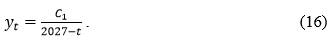
It is not difficult to see that this formula is virtually identical with the law of the hyperbolic growth of the Earth population discovered by von Foerster in 1960 (see Eq. (15) above and below):

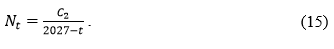
It is easy to see that these two equations only differ with respect to the value of parameter C in the numerator.

Note, however, that this acceleration pattern is not trivial at all. In the meantime, it appears important to note that, notwithstanding some fundamental similarity, the pattern of the planetary macroevolutionary acceleration (that can be traced in the Panov and Modis – Kurzweil series) differs substantially from the pattern discovered by von Foerster with respect to the world population growth.

The point is that у of Eq. (16) is the global complexity growth rate, that is why equation y = C₁/(2027–t) does not describe the growth of the global complexity; it describes precisely the increase in the global complexity growth rate. And, that is why у of Eq. (16) does not correspond to the world population (N) of Eq. (15); it corresponds to the world population growth rate; whereas the equation describing the growth of the world population (N) differs substantially from the equation describing the dynamics of the world population growth rate (dN/dt).

Indeed, as we remember, algebraic equation of type

can be regarded as the solution of a differential equation of type

Thus, if the world population grows according to the following law:
N = C₂/(t*–t) (14), its growth rate will follow a rather different law:

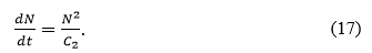
On the other hand, substituting N with C/(t* – t) in dN/dt = N²/C we get

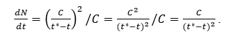
Thus, the world population grows^[38] following the simple hyperbolic law

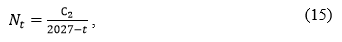
whereas the world population growth rate increases following the quadratic hyperbolic law:

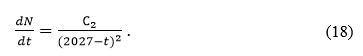
Compare this now with equations describing the growth of global complexity. Let us (with Fomin 2020 and Panov 2004, 2005a, 2005b) denote the global complexity level as n.^[39] With such an approach, the above-mentioned variable y may be denoted as dn/dt. As we remember, the global complexity growth rate (y = dn/dt) increases in the Panov series^[40] following the law that is substantially different from the equation describing the dynamics of the world population growth rate (18):

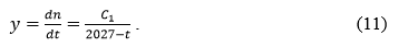
Note that the solution of differential Eq. (11) looks as follows:

where А is a constant.^[41]

Thus, the growth of planetary complexity (n) follows the law that is rather different from the one followed by the world population (N) growth (see Tab-
le 1):

Table. Comparison between equations describing the planetary complexity growth, and the world population growth

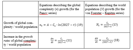
As we see, the world population (N) grew (until the early 1970s) following a simple hyperbolic law (N_t = C/t* – t), whereas the global complexity was increasing following a logarithmic hyperbolic law (n_t = const – C∙ln(t* – t)).

On the other hand, the world population growth rate (dN/dt) changed (until the early 1970s) following a QUADRATIC hyperbolic law (dN/dt = C/(t*–t)²), whereas the global complexity growth rate was increasing following a SIMPLE hyperbolic law (dn/dt = С/t*–t).

Nevertheless, the question remains – is this a coincidence that (until the early 1970s) the global complexity growth RATE (dn/dt) in the Panov series and the world population (N) were increasing following the same law: x_t = C/(2027–t)? Note that calculations performed below by Alexey Fomin (2020) suggest that this might not be a mere coincidence.

Indeed, Alexey Fomin (2020: Ch. 5) brings our attention to the point that during the social phase of the Big History / Universal Evolution, the population of the Earth between each pair of ‘biospheric revolutions’ increased about the same number of times (somewhere around 2.8). Moreover, Fomin (Ibid.: 89) demonstrates mathematically that against this background ‘the increase of the world population by a factor of α is accompanied by the reduction of duration between phase transitions by the same factor of α’. That is, if between the biospheric revolutions the population on average increases by a factor of α, then (against the background of hyperbolic growth of the world population) the intervals between each subsequent pair of biospheric revolutions will be reduced by a factor of α. (It appears appropriate to recollect at this point that this coefficient α is nothing else but what Panov [2005a: 128] denotes as ‘a coefficient of acceleration of historical time’ and ‘a coefficient of reduction of the duration of each subsequent evolution phase’^[42] [Idem 2005b: 222]). At the same time, Fomin's (2020) empirical calculations confirm that the average value of the increase in population between biospheric revolutions is approximately equal to the average value of the shortening of the time periods between biospheric revolutions. His (Ibid.) calculations show that both values are located within the interval 2.5–2.8, which is close enough to the value of α, empirically calculated by Panov (2,67, see, e.g., Idem. 2005a: 130; 2005b: 222).

However, Fomin's (2020) own explanation why ‘the increase of the world population by a factor of α is accompanied by the reduction of duration between phase transitions by the same factor of α seems to be a bit difficult to comprehend (though in no way it can be called wrong). So, below I will try to explain the respective regularity in a simpler way.

The hyperbolic growth of the world population (observed till the early 1970s) meant that it grew according to the following law:

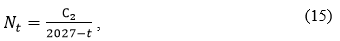
that can be also expressed as

where x is the time until the Singularity (x = 2027 – t). The very nature of the hyperbolic growth implies that in order that the world population (N) could increase by a factor α (e.g., 3 times), the time till the Singularity should decrease precisely by the same factor α (that is, the same 3 times in our case). As a result, each new period of multiplication of N by a factor α (e.g., population tripling) will be shorter than the previous multiplication period (e.g., the previous period of population tripling) by the same factor of α (in our case – three times). However, if each period of multiplication of the world population by some factor α is accompanied by a ‘complexity jump/phase transition’ (as has been demonstrated by Fomin [2020]), then the length of this period turns out to be just the reciprocal of the global macroevolution rate (that is defined as the frequency of phase transition per unit of time) – thus, each increase in the size of the world population N by the factor of α should be accompanied by the increase in the global complexity growth rate (y = dn/dt) by the same factor of α. Thus, we find that, against the background specified above, the dynamics of the world population (N) and the global complexity growth rate (dn/dt) should be described by the same equation (5) (albeit, of course, with different values of parameter C).

In other words, already from the fact that the average value of the population increase between biospheric revolutions is approximately equal to the average value of the shortening of time between biospheric revolutions, it follows that the growth rate of global complexity (dn/dt) should be proportional to the population of the Earth (N), and therefore N and dn/dt must grow according to one law. Indeed, as has been shown above, if N has increased by a factor of α, then the distance to the next biospheric revolution must be reduced by a factor of α, too. But we calculate the growth rate of global complexity (dn/dt) just as ‘1’ divided by the number of years between biospheric revolutions (which gives us ‘the number of biospheric revolutions per year’). Thus, the reduction of time between biospheric revolutions by a factor of α means by definition that the intensity of the global macroevolution rate (dn/dt) should increase by the same factor of α. This means that if the increase of N by a factor of α is accompanied by a reduction in the time between biospheric revolutions by a factor of α, and the reduction of the time between biospheric revolutions by a factor α increases the intensity of the global macroevolution (dn/dt) by a factor α, then the increase of N by α times should be accompanied by an increase in dn/dt by a factor of α, which means that N is proportional to dn/dt, and they grow according to one law.

Now let us demonstrate this more formally. Since the movement from one biospheric revolution to another is accompanied by an increase in population N by the same factor of α and an increase in the index of global complexity n by one unit, we obtain:

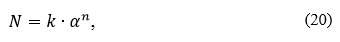
where k is a coefficient of proportionality between N and αⁿ.^[43]

Taking into account that

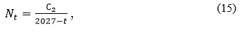
we arrive at:

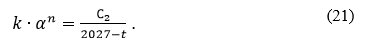
This implies the following:

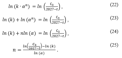
Differentiating expression (25), we obtain:

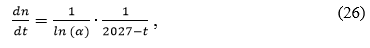
or

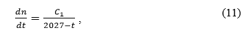
where С₁ = 1/ln(α).^[44]

Thus, we obtain analytically that if the world population (N) grows hyperbolically according to the law N_t = C₂ / 2027 – t, whereas the ratio N = k∙αⁿ is observed between the index of global complexity (n) and the population of the Earth (N), then the global complexity growth rate (dn/dt) will increase according to the same hyperbolic law (x = C / 2027 – t) as the population of the Earth. The tests whose results are presented in this chapter demonstrate that these theoretical expectations find an unexpectedly strong empirical support (at least,
I myself did not expect it to be so strong).

So, the calculations suggest that the fact that, up to the beginning of the 1970s, the world population SIZE (N) and the global complexity increase RATE (dn/dt) in the Panov series grew following the same law (x_t = C / 2027 – t), is by no means a coincidence; it is rather a manifestation of a fairly deep pattern of the global evolution. Thus, at the social phase of universal and global history, the hyperbolic growth of the rate of increase in global complexity and the hyperbolic growth of the Earth's population are two closely related aspects of a single process.

It should be noted that this is not in bad agreement with many mathematical models of hyperbolic growth of the world population^[45], as such models tend to consider the hyperbolic growth of the world population as a result of the functioning of the positive feedback mechanism of the second order between demographic growth and technological development, when technological development (most vividly manifested precisely as ‘biospheric revolutions’ – e.g., the Neolithic Revolution, or the Industrial Revolution) significantly accelerated the growth rate of the population, which (by virtue of the principle ‘the more people, the more inventors’^[46]) through collective learning mechanisms accelerated onset of each successive ‘biospheric revolution’ (that usually corresponded to a new major technological breakthrough). In particular, this correlates very well with an idea that was developed long ago by Taagepera (1976, 1979), Kremer (1993), Podlazov (2000, 2017), and Tsirel (2004) who demonstrated that the global technological growth rate is to be proportional to the global population, and who explained the hyperbolic growth of the world population through this point.

Thus, ‘the growth rate of technology is proportional to total population (Ibid.: 682). We have already mentioned that for the human part of the Big History the ‘complexity jumps/biospheric revolutions’ identified by Modis and Panov correspond rather closely to the major technological breakthroughs in the human history (see Grinin et al. 2020: Ch. 14); hence, for the human part
of the Big History the global evolutionary macrodevelopment rate detected
in their series can well be regarded as a proxy for the global microtechnological development. Thus, already the theory developed by Taagepera, Kremer, Podlazov, and Tsirel would allow to expect that for the human part of the Big History we should find a rather high correlation between the size of the world population and the global evolutionary macrodevelopment rate. However, I am sure that Taagepera, Kremer, Podlazov, and Tsirel themselves will be a bit surprised to see that their theoretical expectation finds such a strong support
(r = 0.997, p < 0.001) for a test employing an apparently rather imperfect proxy of the global technological growth rate (see Fig. 1):

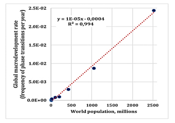
Fig. 1. Correlation between the world population and the global macrodevelopment rate in the Panov series, scatterplot with a fitted regression line, natural scales

Source of data on the historical world population estimates: Kremer 1993: 683.

In the double logarithmic scale this correlation looks as follows (see Fig. 2):

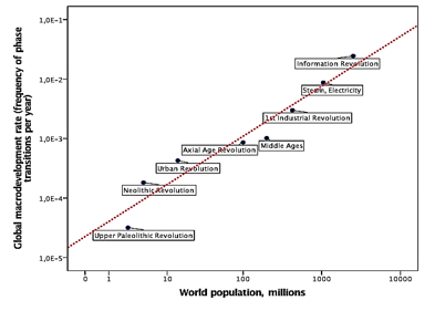
Fig. 2. Correlation between the world population and the global macrodevelopment rate in the Panov series, scatterplot with a fitted regression line, double logarithmic scale

Source of data on the historical world population estimates: Kremer 1993: 683.

Note that we still obtain rather similar results when we use estimates developed more directly to measure the global technological growth rate. Grinin et al. (2020: Ch. 14) attempt to estimate specifically the dynamics of the global technological growth rate by identifying the main phase transitions in the specifically technological macrodevelopment (see also Grinin 2006). It is highly remarkable that the resultant series of estimates of the global microtechnological growth rates turn out to be described with very high accuracy by an equation of type (5) that describes so well both the macrodynamics of the world population and the planetary complexity growth rate (see Grinin et al. 2020: Ch. 14). Against this background, it is hardly surprising to see that this series of specific estimates of the global technological growth rates demonstrates a comparably high correlation with the world population size (r = 0.992, p < 0.001), especially for the period since the start of more reliable estimates of both the world population and global technological growth rates and till the beginning of the systematic decline of the world population growth rates (see Fig. 3). This correlation with double logarithmic scale is presented in Fig. 4.

It is of a special interest that Grinin's series (Ibid.) demonstrates such properties that are rather similar to the ones that were found by Fomin below (see Fomin 2020: Ch. 5) with respect to Panov's series – the population of the Earth between each pair of phase transition tended to increase about the same number of times (α), whereas the periods between technological phase transitions tended to decrease by the same factor of α. Note, however, that Panov singled out primary phase transitions, whereas Grinin's list includes some secondary phase transitions. Consequently, for the period since the Agrarian (Neolithic) Revolution Grinin identifies almost twice as many phase transitions as Panov. As a result, for the Panov series the value of α turns out to be close to Euler's number (e), whereas for the Grinin's series it appears closer to the square root of Euler's number (√e).

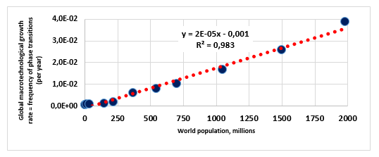
Fig. 3. Correlation between the world population and the global macrotechnological growth rate, 8,000 BCE – 1950 CE, scatterplot with a fitted regression line, natural scales

Source of data on the historical world population estimates: Kremer 1993: 683; source of data on the historical estimates of the global macrotechnological growth rate: Grinin 2006; Grinin et al. 2020: Ch. 14.

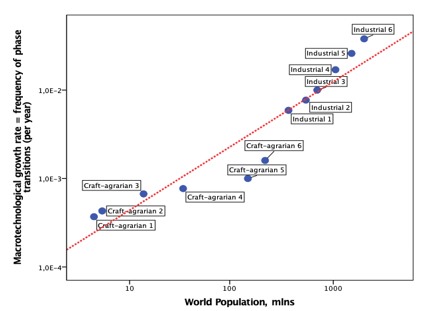
Fig. 4 Correlation between the world population and the global macrotechnological growth rate, 8,000 BCE – 1950 CE, scatterplot with a fitted regression line, double logarithmic scale

Source of data on the historical world population estimates: Kremer 1993: 683; source of data on the historical estimates of the global macrotechnological growth rate: Grinin 2006; Grinin et al. 2020: Сh. 19.

Appendix 2.
On Some Patterns on Global Macroevolutionary
Acceleration. Additional Calculations

As has been shown by Alexander Panov^[47], for his series of ‘biospheric revolutions’ one can observe the following regularity:

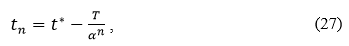
where ‘the coefficient α > 1 is a coefficient of reduction of the duration of each subsequent evolution phase comparing with the corresponding preceding one.
T is a duration of the whole period of time under consideration^[48], n is a number of phase transition, and t* is the limit of the geometrical progression {t_n} and t* may be called as singularity of the evolution’ (Panov 2005b: 222; see also Panov 2005a: 128). Note that, as we have shown above, n can also be well interpreted as a global complexity index.

For further calculations, Panov (2005a: 129; 2005b: 222) transforms Eq. (27) along the following lines:

However, below Alexey Fomin (2020; Ch. 5) shows that for a further analysis of the Panov model it is better to use a slightly different version of the transformation of Eq. (27):

Indeed, Eq. (29) can be rewritten as follows:

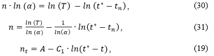
where А = ln(T)/ln(α), аnd С₁ = 1/ln(α).

At the same time, as we recall, the algebraic equation (19) is a solution of the following differential equation:

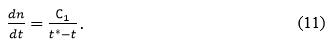
Thus, we obtain the same equations (19) and (11), which were obtained by us earlier in a somewhat different way.

Note that Panov's calculations indicate that the value of α equals 2,67, which, as Panov notes, turns out to be very close to the numeric value of the mathematical constant e / Euler's number (2,718…), and one cannot exclude
the ‘coefficient of acceleration of historical time’ could turn out to be actually so close to Euler's number that the parameter α in equations (11), (31) and (20) may be replaced with e. In this case, the set of equations describing the hyperbolic acceleration of global macroevolutionary development rate appears particularly elegant in its simplicity. Indeed, taking into consideration the point that in the equation

А = ln(T)/ln(α), and С₁ = 1/ln(α), when substituting e, instead of α, we arrive at

Taking into account the point that in the equation

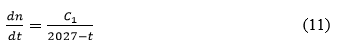
С₁ = 1/ln(α), when substituting e, instead of α, we arrive at

In addition, the equation

when substituting e, instead of α looks as follows:

from which it follows that

As a result, the set of equations describing the hyperbolic acceleration of the global macroevolutionary development rate turns out to be especially elegantly simple:

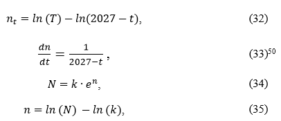
where, let us recollect, n denotes the global complexity index, T is the period of the existence of the life on the Earth (~ 4 billion years), N is the world population, and k is a constant.

However, it appears difficult not to agree with Alexander Panov that ‘the question whether the point [that the value of coefficient α is so close to e] has any deep sense remains open’ (Panov 2005a: 130).

^[1] Actually, a prototype of this figure (but in a double logarithmic scale) was reproduced by Kurzweil already in 2001 in his essay ‘The Law of Accelerating Returns’ (Kurzweil 2001: 5).

^[2] And with a slightly different calculation mode than the one that we will apply below, the denominator of this equation will be a number that is slightly different from ‘1’.

^[3] To be more exact, this is the date, when according to the most recent Kurzweil forecast, the humans will become immortal, which still can well be considered as a sort of singularity (as well as a rather valid candidate for the possible dating for Threshold 9 of the Big History) – even if we actually deal with the radical increase in the human (or posthuman?) life expectancy rather than with the immortality per se, as this would still imply the change of the biological nature of the humans, which cannot but affect the course of the human history in a rather dramatic way.

^[4] His calculations described below were first presented in November 2003 at the Academic Seminar of the State Astronomic Institute in Moscow (Nazaretyan 2005: 69) and subsequently published in his articles (Panov 2004, 2005a, 2005b, 2006, 2011, 2017) and monograph (Panov 2008).

^[5] Note that the left-hand diagram was only presented by Panov at the Academic Seminar of the State Astronomic Institute in November 2003, whereas in his printed works he only reproduces the right-hand diagram, using another visualization of the global macrodevelopment acceleration for the whole of the global history since 4 billion BP. On the other hand, the left-hand diagram was reproduced in print by Akop Nazaretyan (2015a: 357; 2018: 31) with reference to Panov.

^[6] See Fig. 6 above.

^[7] See Fig. 6 above.

^[8] Or, to be exact, 2.054.

^[9] Modis first presented his results in the article in Technological Forecasting and Social Change (that Panov only read in March 2018 after it was sent to him by me) in 2002, whereas Panov first presented his results next year at the Academic Seminar of the State Astronomic Institute in
Moscow.

^[10] Actually, Modis starts with the ‘Big Bang’; however, Kurzweil, quite reasonably, prefers to start the series with the origins of the Milky Way.

^[11] A more popular version of Modis presentation (2003) appears to contain a misprint indicating 19,200 years ago as the date of the invention of agriculture. This misprint is absent from the more academic version of Modis presentation (2002), on which we rely at this point.

^[12] This book is also available in English (Diakonov 1999).

^[13] Without providing any exact references.

^[14] Without providing its URL.

[15] URL: http://drnelson.utmem.edu/evolution2.html.

^[16] At least when preparing his first list of ‘phase transitions/biospheric revolutions’ in Russian (Panov 2004, 2005a). Note that when preparing the publication of his results in English Panov (2005b) added to his originally overwhelmingly Russian bibliography eight references in English (Begun 2003; Carrol 1988; Jones 1994; Nazaretyan 2003; A.H. 1975; A.P. 1975; J.B.W. 1975; T.K. 1975) and one reference in German (Jaspers 1955). One cannot exclude that this might have affected some of Panov's datings of some of his ‘biospheric revolutions’ (there are indeed some slight differences in datings between Panov 2005a and Panov 2005b). Note that these new references included four articles in Encyclopedia Britanica, which made the list of sources in Panov 2005b not as perfectly different for Modis' list as the list of sources in Panov 2005a (because Modis also lists Encyclopedia Britanica among his list of sources). So, for the sake of ‘the purity of experiment’ we decided to rely for our calculations on Panov's list of ‘phase transitions’ provided in his original publication of his results in Russian (2005a) rather than in English (2005b).

^[17] Though one of his sources (Heidmann 1989) is a translation into English of a book originally written in French.

^[18] The description of Panov's phase transitions / ‘biospheric revolutions’ have been taken from 2005 Panov's presentation of his findings in English (Panov 2005b: 221); however, the datings of those phase transitions are from the earlier Russian version (Idem. 2005a); I indicate explicitly the difference between those datings when it is observed. Note that for our calculation below we have used the datings from Panov 2005a (not Panov 2005b). In cases when Panov (2005a) indicated time ranges rather than exact time points, we have used middle values for our calculations – for example, Panov (2005a) indicates as the date of his ‘biospheric revolution 5’ (‘Hominoid revolution / The beginning of the Neogene period’) 25–20 · 10⁶ years ago, whereas for our calculations we use the intermediate value for this time range (22.5 · 10⁶ years ago).

^[19] 570 · 10⁶ years ago according to Panov 2005b.

^[20] 24 · 10⁶ years ago according to Panov 2005b.

^[21] 4–5 · 10⁶ years ago according to Panov 2005b.

^[22] 2–1.5 · 10⁶ years ago according to Panov 2005b.

^[23] 0.7 · 10⁶ years ago according to Panov 2005b.

^[24] 750 B.C. according to Panov 2005b.

^[25] A.D. 500 according to Panov 2005b.

^[26] A.D. 1500 according to Panov 2005b.

^[27] 1830 according to Panov 2005b.

^[28] Note that the power-law regression that produced this value for the world populations series had been performed more than 50 years before a similar regression produced the same value of t* for the Panov series (actually, the first regression was performed before the birth of the author of the present article). Still I would not take too seriously such astonishingly similar values of t* parameter produced by different power-law regressions for very different time series in very different years; of course, there is a very high degree of coincidence here. In any case, as we will see below, there are no grounds at all to expect anything like Doomsday on Friday, November 13, A.D. 2026.

^[29] Note that all the calculations below of the world population are conducted in millions. Note also that the value of parameter С used by us is a bit different from the one used by von Foerster.

^[30] This is done, e.g., by Nazaretyan (2015a, 2018).

^[31] While demonstrating that the resultant singularity should be interpreted as an indication of an inflection point, after which the pace of global evolution will begin to slow down systematically in the long term.

^[32] Incidentally, this is very close to the singularity of 2005 CE that we detected earlier for Maddison (2007) series of the world GDP estimates (Korotayev, Malkov, and Khaltourina 2006a, 2006b; Korotayev and Malkov 2016), and that was detected even much earlier for the same date by Rein Taagepera (1976) in the world GDP estimates available to him by that time.

^[33] This roughly corresponds to Big History Thresholds 5, 6, and 8.

^[34] And, thus, at least three more Big History Thresholds.

^[35] The earliest attempt to detect mathematically the singularity on the basis of data from the human history seems to have been undertaken in 1909 by Henry Adams who found it for year 1921 according to one version of calculations, and, according to the second version of his calculations – for 2025 CE (Adams 1969 [1909]: 308) – incidentally not so far at all from 2027 CE detected by Heinz von Foerster in 1960, and by us in the Panov series just above.

^[36] Note that for the detection of the singularity in his series Grinchenko applied a methodology that was somehow different from the methodologies used either by Panov or by me above.

^[37] I would like to express my deep gratitude to Sergey Shulgin and Alexey Fomin for their invaluable help with the calculations contained in Appendices 1 and 2.

^[38] Or, to be more exact, it grew this way till the early 1970s.

^[39] Note that within this perspective the level of planetary complexity at a given time will be calculated by the number (n) of ‘biospheric revolutions’ (according to Panov – Fomin) or ‘complexity jumps’ (according to Modis) – based on the assumption that every ‘complexity jump’ adds to the present n one more level of complexity.

^[40] Note, however, that within the Modis – Kurzweil series the global complexity growth rate increases following the same law (with a slightly different values of parameters С₁ and t*).

^[41] Incidentally, the calculations performed by Alexander Fomin (2020: Ch. 5) allow to identify the value of this constant for the Panov series. It turns to be equal to lnT/lnα, where T is the period of the existence of life on the Earth (that can be estimated as ≈ 4 billion years), and α is ‘a coefficient of acceleration of historical time’ (Panov 2005a: 128) / ‘a coefficient of reduction of the duration of each subsequent evolution phase’ (Panov 2005b: 222). For more details on the coefficient α see below (in particular, Appendix 2).

^[42] That is a period between ‘biospheric revolutions’ / ‘complexity jumps’. – A.K.

^[43] Note that an empirical test performed by Alexey Fomin (2020: Ch. 5) supports the hypothesis of the presence of this non-trivial relationship.

^[44] Note that, among other things, our calculations allow us to establish analytically the value of the parameter C₁ in Eq. (11).

^[45] See, e.g., Korotayev, Malkov, and Khaltourina 2006a, 2006b; Taagepera 1976; Kremer 1993; Podlazov 2000, 2001, 2002; Tsirel 2004; Korotayev and Malkov 2012; Korotayev 2012, 2013; Korotayev and Malkov 2016; Grinin, Markov, and Korotayev 2013, 2014, 2015.

^[46] As Kremer puts it, ‘high population spurs technological change because it increases the number of potential inventors… In a larger population there will be proportionally more people lucky or smart enough to come up with new ideas’ (Kremer 1993: 685–686). Kremer rightly notes that ‘this implication flows naturally from the nonrivalry of technology… The cost of inventing a new technology is independent of the number of people who use it. Thus, holding constant the share of resources devoted to research, an increase in population leads to an increase in technological change’ (Ibid.: 681). Note that we are dealing here with a mechanism that is actually identical with what David Christian denotes as ‘collective learning’ effect (Christian 2005).

^[47] See, e.g., Panov 2005a, 2005b and Panov 2020: Ch. 20.

^[48] As mentioned above, T can be considered as the time of existence of life on Earth and equated to ≈ 4 billion (years).

^[49] Note that Fomin's calculations (Fomin 2020: Ch. 5) indicate that if, in calculating with the help of Eq. (11), t is taken not as the moment of the beginning of the period by which the derivative is calculated, but as its middle, then the value of the parameter C₁ turns out to be closer to 1 rather than to 2. See also Widdowson 2020: Ch. 22.

^[50] Note that this equation is virtually identical with the one presented by Kurzweil (2005: 23) in his graphic explanation of the notion of mathematical singularity (see Fig. 2 above).