The Trajectory of the World System over the Last 5000 Years

Almanac: History & Mathematics: Processes and Models of Global Dynamics
Abstract
That history has a path, a trajectory through time, has been the focus of study by many prominent scholars including Marx (1977), Toynbee (1946), Jaspers (1965), Diakonoff (1999), and others. It is the intent of this paper to delineate this path as a trajectory of the world system through time. The term "world system" is used here as initially defined by Wallerstein (1974) and then modified by Modelski (2003) to represent a single, global, world system. This paper addresses the problem of delineating the trajectory of the world system from a more quantitative and mathematical perspective than has previously been done.
Assuming that urban areas through time have a Pareto-like distribution, a mathematical model relating the magnitude of the total world system population, T, the ratio of largest to smallest urban area, a, and γ, a measure of the form of the distribution and also a proxy for the connectedness of the distribution, is constructed. The model is used to graphically represent all possible states of the world system and to plot the actual position of the world system through time. The actual trajectory has some notable large scale characteristics which are discussed. Other smaller scale trends are also noted.
A partial analysis of the constraints limiting this system is given and includes a consideration of the magnitude of changes in each of the model variables, the relationship between changes in the variables, α and C, of the distribution of urban areas, and a consideration of the relationship between γ and future values of that variable removed by one, two, or three centuries. The (apparent) scale-free nature of the model is also assessed. Finally, it is noted that the analysis of residuals of the linearized relationships between γ and both T and a yield cyclical changes with very long term periodicity.
Keywords: world system, math model, mixed strategy, Pareto-like distribution, search-pattern, theoretical space, urbanization.
Introduction
The concept of a world system as first envisioned by Immanuel Wallerstein (1974) consists of a single or small group of core polities connected economically to a larger number of semi-peripheral polities which are in turn econo-mically connected to an even larger number of peripheral polities. The core polities exploited the semi-peripheral and peripheral polities with respect to resource extraction, and were the center of production of this pyramidal organization, this production being driven by global capitalism. Wallerstein (2004) defines capitalism as continual or endless consumption with the implication that there will be an on-going flow of materials from peripheral and semi-peripheral polities to the core producers. It should be noted here that this arrangement of core to peripheral polity is analogous to a Pareto-like distribution in which high frequency entities are members of low magnitude classes, in this case low magnitude classes have low access to wealth, and low frequency entities have access to considerable wealth.
Since the inception of the world system concept other scholars have investigated the reality of the existence of the world system over the course of human history and have charted the historical paths of this system. Notable among these scholars are the late Andre Gunder Frank and William Thompson (2005), as well as George Modelski (2003). Also deserving note for their work on macro-models of world system behavior are Andrey Korotayev, Artemy Malkov, and Daria Khaltourina (2006a, 2006b; Korotayev and Khaltourina 2006). Their work, led by Korotayev, has taken a detailed look at both contemporary phenomena such as the global demographic transition we are currently rapidly approaching and the Medieval and contemporary demographics of Africa and also the historical demographics of Medieval Egypt, always with the concept of the world system providing the fundamental direction for their work. Also of note is Historical Dynamics by Peter Turchin, a work that addresses the mathematical study of dynamic changes in agrarian polities, particularly secular cycles, and encompasses almost the entire time period under study in this paper.
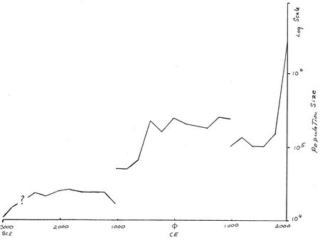
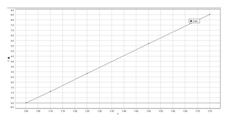
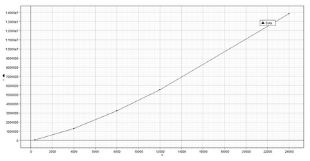
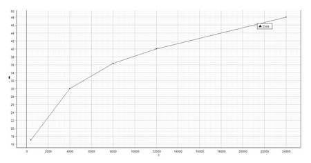
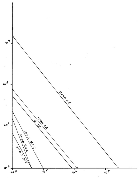
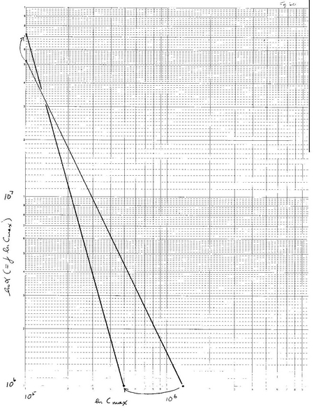
Of the scholars mentioned George Modelski (2003 and elsewhere) has taken the broadest view of world system evolution and history and has provided a graphical model of world system evolution as it is reflected by both changes in urbanization and changes in global population magnitude. His model, a graph of five thousand years of world system history, consists of phases of growth punctuated by phases of reorganization, with each phase lasting about one thousand years. While the phases of growth are characterized by a positive slope, the periods of reorganization are plateau-like with an average slope of zero (see Figures 1a and 1b). The form of these graphs themselves can be produced either by tracking the global population of the world system over time or by tracking the maximum size of urban area over time. In either case the same pattern is produced, that pattern being a set of two plateaus flanked by by periods of directed change and characterized by more or less continuously decreasing values of γ. For the purposes of this paper Modelski's data on world cities have been modified to produce Figures 1a and 1b. Specifically, the minimum total number of people inhabiting world cities for the Ancient, Classical, and Modern World systems by taking the number of world cities and multiplying that number by the average minimum number of people inhabiting those cities as defined by Modelski (2003). Figure 1a is a punctuated linear plot of this data in which each segment represents each of the three historic periods. It can be seen that the first two segments of this graph have essentially the same shape even though the city size differs by an order of magnitude. The segment of this graph representing the Modern World system has the form of an exponential curve. In Figure 1b the ordinate is logarithmic, and the sense of scale between the three ages gives a clearer picture of the relationship between the periods of growth and the plateaus, designated as periods of reorganization by Modelski. Of interest is the fact that the period of time known as the so-called Dark Ages, i.e. the early Medieval Age, is associated with one of the phases of reorganization and such events as the ends of the Early, Middle, and Late Bronze Ages are associated with an earlier period of reorganization.
This paper proposes to investigate world system behavior over time, i.e. world system evolution, from a more quantitative and mathematical perspective. Included within this analysis will be the assessment of the degree of connectedness of the world system as it is reflected by urbanization. It is the intent here to map out the limits to or constraints on world system evolution, and the approach to this evolutionary analysis is not unlike that of Raup and Michelson (1965) in which they established physical constraints to the evolution of the molluscan coiled shell.
Fundamental to this approach is the construction of a model based on appropriate assumptions regarding the structure, function, and evolution of the world system. These assumptions must not only constrain and guide the form of the model constructed but also permit modifications to the model. Further, these assumptions will define the ability of the model to reflect reality, generality, and precision with respect to the function of the model. Recall that only two of the three model characteristics can be satisfied by any given model. The model constructed in this analysis has considerable generality having general applicability over time and is capable of making precise predictions, but does not reflect any particular reality, i.e. it is global in scope. In other words, the model will not represent the detailed historical course of the Roman Empire, or the demise of the Mayans, or the migrations of the Xiongnu. Rather, it will provide a specific context within which specialists can research the details of these and other civilizations. Finally, because of the nature of this model, it should be considered as a complimentary and supplementary tool to other types of historical research, not a replacement of standard historical scholarship; the domain of historical research is being expanded rather than shifting its locus.
Figure 1a. The left-hand ordinate represents the number of world cities of the Ancient World, while the right-hand ordinate represents the number of world cities in the Classical World with the upward right-pointing arrow representing the increase in world cities of the Modern Age.
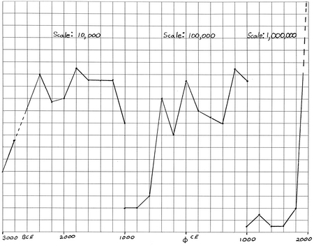
Figure 1b. This graph is a semi-logarithmic representation of the data depicted in Figure 1a. The scale of the minimum total populace living in world cities for each of the ages represented reveals a difference by an increase in an order of magnitude as one progresses through the five thousand year period to the present. Note that the question mark at 2600 BCE represents a lack of available data. The ordinate scale in the following successive orders of magnitude, 104, 105, and 106, all representing population size.
The model
The intent of this model is to provide a tool by which parameters can be generated that characterize the state of the world system with respect to the degree of urbanization, the magnitude of the world system population, and the degree of connectedness of the world system. The model depends on three fundamental assumptions, first, that a world system does in fact exist and has existed over historical time and is global in extent, an assumption that is on (reasonably) solid ground, second, that the distribution of urban areas is Pareto-like, i.e. as described in the Introduction, that there are many urban areas that are small, while there are a few large urban areas, and, third, that the distribution is scale free. Explicitly, this distribution can be described by the following equation:
F = αC-γ, (1)
where F represents frequency, α represents the maximum size of an urban area raised to the (positive) gamma power, C represents the class size of a given urban area as measured by its population, and γ is the exponent and is a measure of connectedness between urban areas as per the third assumption.
The total population of the world system, T, is then the sum of the world system urban population Tu, and that portion of the population existing rurally, Tr. An equation can be derived (see Appendix for the relevant mathematics) which relates the ratio of largest to smallest urban size, a, the global population, T, and gamma, γ, the exponent of Eq. 1, which represents the degree of connectivity between urban areas. This equation is:
aγ C0γ – 1 – a – (γ – 1)T/ C0 = 0 (Eq. 18 of the Appendix)
Note that the symbol, C0, represents the smallest urban size and is held constant in value at 100. It should also be apparent that Eq. 18 has a single dimension, population number, in this case of people. In other words, while a and the ratio, T/C0, are dimensionless, C0 is not; it has the dimension noted above. Data for both T and the maximum urban area size over the last five thousand years (Chandler 1987; Modelski 2003; and the US Census Bureau), and then γ may be computed. Using the values of γ, T, and a = Cmax/C0 acquired from the data set mentioned above, the state of the world system can then be plotted over the last five thousand years. However, Eq. 18 may also be used to generate a plot of all possible states of the world system, and this plot may then be used in comparison with the actual plot mentioned previously to determine what combinations of γ, T, and a are permissible and what are not. The question may then be posed: Why are certain sets of γ, T, and a functional while others are not? First, however, it will be important to generate the theoretical landscape.
The theoretical landscape of the world system
The theoretical surface generated by Eq. 18 (see Figure 2) represents a surface in three-space with the axes x = a, y = γ, and z = T/C0. However, the log transform of Eq. 18, ln[aγC0 γ-1 – a] – ln[(γ – 1)T/C0] = 0, is to be used here so that the data having lower orders of magnitude could be displayed appropriately. For instance, the global population at 3000 BCE has been estimated at fourteen million, whereas one thousand years later it is twenty-seven million, and a thousand years further on, fifty million. In that same period of time the maximum urban size changes from forty thousand to eighty thousand in 2800 BCE and 2300 BCE and then to one hundred thousand by 1000 BCE. If, however, the span of the Common Era is considered, i.e. the last two thousand years, the global population changes from approximately one hundred and seventy million to over six billion and in the same period of time the maximum urban size increases from eight hundred thousand to over twenty million. Representing this last set of figures dwarfs the other data, e.g. by a factor of five hundred with respect to the maximum urban area of 3000 BCE. It should also be kept in mind that the surface in Figures 2, 3, 4, and 5 was determined by computing the zeros for Eq. 18. Also, when doing so the upper and lower bounds for a, γ, and T were determined empirically, specifically they are: 400 < a < 23,000, 1 < γ ¸1.6, and 14,000,000 < T < 6,000,000,000.
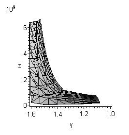
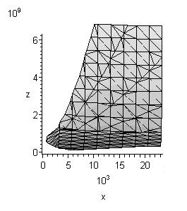
Figure 2. This figure represents the surface of Eq. 18, i.e. the theoretical surface of the world system in three dimensions. The x-axis represents the magnitude of the variable, a, the y-axis represents the magnitude of gamma, and the z-axis represents the magnitude of the variable, T.
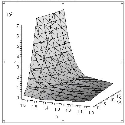
This surface exhibits some important characteristics. It is in general L-shaped with a slight downward crease toward low values of T and a and higher values of γ. The upright portion of the L-shape is a surface that slopes steeply toward a sharp boundary with the horizontal portion of the L-shape. The angle of this junction will become clear in the view of γ v. T in Figure 4 which reveals a very clear L-shape. In Figure 3, γ v. a, the shape appears fan-like, and in Figure 5, a head-on view of the surface a similar fan-like appearance is revealed. In the following section it will be clearly shown that, while this surface is considerable, the portion actually occupied by the world system over the last five thousand years is quite restricted.
The morphology of the world system three-dimensional landscape will now be considered in terms of three plane views, that of x-y, z-y, and z-x as represented in Figures 3, 4, and 5. Viewed in the x-y plane, i.e. a plane representing a plot of γ v. lnT, the entire plane is occupied with two notable features, the aforementioned upright and horizontal portions of the L-shape and also an attenuation of the horizontal member as γ approaches one. In the y-z or γ v. lnT/C0 plane the plot represents the distinctly L-shaped form with the previously mentioned attenuation. In the a – lnT/C0 plane the plot reveals a distinct fan-shape with the attenuated portion of the graph extending toward the viewer.
Figure 3. This figure represents a two-dimensional view of the theoretical landscape representing only the magnitudes of gamma and a. The y-axis representing gamma is horizontal, and the axis representing a is vertical. Note that as a increases, gamma decreases.
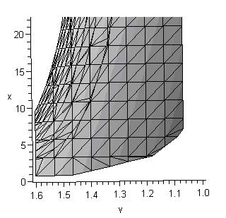
Figure 4. The relationship between gamma (y) and T (x), the world system population, is represented here. Note that the shape of this graph is that of an L and that the horizontal portion attenuates as gamma approaches 1. The general shape of this graph suggests that gamma and T are inversely proportional. The significance of this will be discussed in a later section.
With regard to what a, γ, and T represent in Eq. 18 the morphology of the theoretical surface suggests the following. As global population increases so does urbanization, at least as a broad trend predicted by the nature of this surface. However, in both the case of increase in a or increase in T with respect to γ, γ will decrease. This can be confirmed by considering Eq. 18 where the term (γ – 1)T clearly implies an inverse relation between T and γ, and expressing T as a function of a gives: T = [C0/( γ – 1)][a – aγC0γ-1], where as γ increases, T decreases, and since T and a are directly proportional, then a is inversely proportional to γ.
Figure 5. The relationship between a (x) and T (z) is represented in this figure. While this quadrant is not fully occupied by the surface, it should be apparent by Eq. 18 that a and T are directly proportional.
In summary, the three-dimensional plot of Eq. 18 represents an L-shaped surface with a gradually attenuated horizontal portion. Further, a and T are directly proportional to each other but both are inversely proportional to γ. The significance of this will be addressed in the section "Discussion and implications of the world system trajectory".
The world system trajectory with respect to γ, T, and a
The previous section presented a view of the theoretical landscape of the world system as defined by the equation, aγC0γ-1 – a – (γ – 1)T/C0 = 0. In this section as defined by the data on γ, T, and a listed in Table 1 to be found in the Appendix the actual trajectory of the world system will be described. The description will be given in pair-wise relationships, i.e. a = f(γ), T = f(γ), and T = f(a). In each relationship a graph of the independent and dependent variable will be presented and then discussed.
Figure 6 represents the graph of a = f(γ), where each point represents the position of the world system, and each line connecting points represents the estimated distance that the system took in order to reach the next position in the sequence. This same procedure will be used to represent the remaining two relationships, T = f(γ) and T = f(a). Again, please note that the graph itself is not rectilinear but rather semi-logarithmic, with the abscissa being linear and the ordinate being logarithmic. This is also the case for T = f(γ) but not for T = f(a), as that is double logarithmic relationship. Also note that since time is not represented by either axis but is implicit in the relationship, important temporal landmarks have been represented, e.g. 3000 BCE, the beginning of the plot, 900 BCE, et al.
Figure 6. The trajectory of the world system with respect to gamma, x-axis, and lna, y-axis, exhibits an inverse relationship. There are two broad sub-trends to note here, that there are two periods of oscillation termed search patterns and periods of continuous change in which gamma shows continuous decrease, one extending from the first search pattern to the second, from 300 BCE to 300 CE and from 1800 CE to 2000 CE.
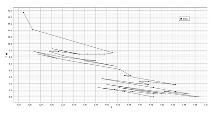
This graph has a number of trends and characteristics which will be noted in turn. The first of these is that there is a broad inverse relationship between gamma and Cmax/C0 (= a). This is predicted by the equation itself and represented in the graphs of the previous section and suggests that any increase in a implies a decrease in gamma, the implications of which will be discussed in the following section. It is comforting however to have empirical data suggest the same trend. However, on a smaller scale there are a number of circumstances where this relationship does not hold.
Within this broad inverse trend between γ and a there are three sub-trends of significance. The first of these is that the graph is not continuous, but is discontinuous with two periods of oscillation between increasing a and decreasing gamma and decreasing a and increasing γ. These oscillatory periods represent considerable periods of time amounting to approximately one thousand years in each instance. Within these periods of oscillation there are segments in which there is no change in abut there is an increase in γ, two in the first oscillatory period bounded by 2500 BCE and 300 BCE, and one terminating the second period and beginning at 1300 CE. The existence of these three anomalous segments suggest that the data represented in Figure 6 are not simply artifacts of aγC0γ-1 – a – (γ – 1)T/C0 = 0. These segments are real and important to the understanding of the world system trajectory.
Punctuating these two periods of oscillation are two (and possibly three) periods of continuous change. The equivocalness of the previous sentence is in all probability an artifact of the available data, however, as graphically represented there are only two pronounced periods of continuous change, one extending from 300 BCE to 300 CE and the current one that is now ending but extends from 1800 CE to the present. A third may exist from 3000 BCE to 2500 BCE, and if so, these three periods of continuous change and two periods of oscillation broadly, and only broadly, conform to Modelski's model of ages of growth interspersed between ages of reorganization. Even so, each period of continuous change represents an increase in a with a concomitant decrease in gamma.
A similar general pattern to that of a = f(γ) of a period of oscillation punctuated with a period of (relatively) continuous increase is evident when considering the graph of lnT = f(γ) (see Figure 7). This pattern is also in overall form an inverse one, i.e. as T increases, γ decreases and vice versa. Over time then γ decreases from a value of just less than 1.6 to one just under 1.25, and during this time, five thousand years, T increases by three orders of magnitude, a condition that may change to four orders of magnitude by the end of this century.
Figure 7. The trajectory of the world system with respect to gamma, x-axis, and lnT, y-axis, is represented here. It should be noted that while the same general trend and sub-trends are represented here as in Figure 6, during the search pattern periods there is a significant horizontal change in gamma with little or no change in T. This would seem to imply that these search-pattern episodes involve change in connectivity with respect to the degree of urbanization but in the absence of marked change in T, i.e. it is as if the world system is being re-packaged without a change in the over-all size of the system.
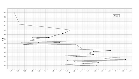
Within this broad inverse trend of increasing T with decreasing γ there are two oscillatory periods, not unlike search patterns, and similar in general form and identical in temporal limits to those noted in a = f(γ), in which there is considerable change in γ with little change in T. Also, the change in γ with respect to T in the graph of T = f(γ) alternated between positive and negative slope, where as the change in γ with respect to a was always negative in the graph of a = f(γ). Each of the search-pattern like structures in Figure 7 is separated by a period of nearly continuous change as they are in lna = f(γ) and of course with the similar temporal limits. The first search pattern extending from 3000 BCE to 1000 BCE includes a period of change in T without any change in γ, so it may be more reasonable to recognize two search-patterns during this time, an older one extending from 3000 BCE to 2000 BCE and a briefer one from 1500 BCE to 1000 BCE. Both of these periods of continuous change represent a change in γ of about –.5. Several so-called Dark Ages are found embedded within these search-pattern periods, the two most notable being the collapse of the Late Bronze Age and the Dark Age (= Age of Reorganization) occurring after the collapse of the Roman Empire.
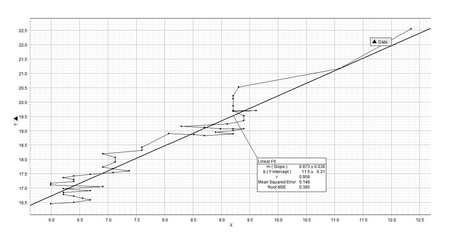
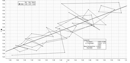
The graph of lnT = f(lna) (Figure 8) differs in general pattern from that of the two previous graphs in that a and T are directly proportional to each other. On a log-log plot the pattern exhibits an essentially linear trend from 3000 BCE with T being approximately 14 million, and a being approximately four hundred to 2000 CE with T being approximately 6.2 billion and a being approximately 23 thousand. However, as in the two previous graphs there are clearly two search-pattern periods, identical in temporal extent to those represented in the two previous graphs, each one associated with the plateaus of the Modelski graph (see Figure 1). As previously noted in the description of the relationship, lnT = f(γ), it is these search-pattern periods that are also associated with periods of so-called societal collapse. Also characteristic of each search pattern is considerable change in awith relatively little change in lnT. There are also two broad periods of continuous change, one extending from 900 BCE to 300 BCE and the second from 1000 CE to the present. Both periods of increase are punctuated by a century of rapid change with essentially no change in lnT. Interestingly, the second such punctuation is actually associated with a slight decrease in lnT.
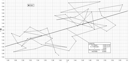
Figure 8a. The relationship between lna, x-axis, and lnT, y-axis, represented here is clearly linear with a positive slope, however, the antilog transform is a power function with an exponent less than one as can be seen in Figure 8b.
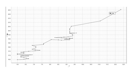
Figure 8b. This is simply the plot represented in Figure 8a fitted with a regression line. As previously noted the antilog transform gives the power function: T = 11.5C.873 (where C is the anti-log transform of the x-axis variable, lnC) which implies that the fraction of the population living in urban settings will increase with increasing T.
It should be noted that the periods of oscillation identified in Figures 6, 7, and 8 of this paper share significant similarities with Figures 7 and 10 of Korotayev and Grinin (2006). Both sets of graphs are double-logarithmic[1] and show oscillatory behavior of the world system over approximately the same period of time, 200 BCE to 1500 CE. However, the graphs in this paper also represent an earlier set of oscillations approximately over the period, 2000 BCE to 1000 BCE. In the Korotayev and Grinin paper the axes are either the logarithm of megacity size or megacity index (x-axis) and the logarithm of developing and mature state area (y-axis). While state area is not represented in Figures 6, 7, and 8, megacity size is and is compared either to γ or to the logarithm of world population. The significance of this similarity is that both sets of graphs represent different aspects of the same underlying process, a process of alternating urbanization and de-urbanization.
Discussion and implications of the world system trajectory
The previous section involved a detailed description of the world system trajectory as it moved through the theoretical three-dimensional space defined by the variables, T, a, and γ. This section will discuss the significance of these trends, offer some explanation of their mechanics, and indulge in some predictions.
From the description of the data it is clear that at least with respect to the three variables, T, a, and γ, and their relationship defined by: aγC0γ-1 – a – (γ – 1)T/C0 = 0, that both T and γ and a and γ are inversely proportional, while T and a are directly proportional. That this is logically consistent is not difficult to show in that if T α 1/ γ and a α 1/ γ, then T α a. However, why should this be in reality? With regard to the function, F = αC-γ, as γ increases F decreases, and if γ represents a measure of connectivity, then it should be expected that as connectivity increases in the world system both T and a should increase, consequently this will only occur as γ decreases. Further, the direct relationship between T and a is intuitively easy to grasp, since urbanization seems to be directly dependent on global population, and, empirically, as T approaches ten billion a larger and larger proportion of T becomes urbanized. This can be shown by Eq. 23 (see Mathematical Appendix for the derivation): Tu/Tr = (a1-γ – 1)/(1 – C0γ-1) (Eq. 23), and by its graph (Figure 9).
Figure 9. The ratio of Tu/Tr, y-axis, with respect to time shows that as a, x-axis, and gamma change over the 5000 year period represented by the data the magnitude of the numerator, Tu, increases as a greater rate than the denominator, implying that the degree of urbanization has increased over time.
Also associated with these broad trends is the fact that the world system trajectory occupies very little space within the bounds of the three variables. What is it then that constrains this trajectory? Clearly, the relationship defined by Eq. 18 may offer some insight, part of which is explained in the following paragraphs, but, for instance, no period of continuous increase spans rather than more than four hundred years, and no period of change in γ occurs over a range greater than .5. Why is this? These questions are posed here so that the remaining paragraphs in this section can be considered within the context of imposed but as yet identified constraints on the system.
As was previously noted, within these broad trends are two sets of patterns, each in all probability dependent on the other. I refer to the two periods of continuous increase punctuated by two periods of what has been labeled as search-pattern behavior on the part of the world system. It is these aspects of world system behavior that will be (partially) analysed here. Also as previously noted the search-pattern periods have embedded within them what Modelski refers to as ages of reorganization. How are these ages of reorganization related to the disjunct search patterns exhibited by the world system trajectory?
These questions will be addressed by assessing each of the following in turn: the magnitude of change of each of the variables with respect to Eq. 18, the rate of change of gamma with respect to gamma itself, the relationship between gamma and preceding gammas, specifically γn+1, γn+2, and γn+3, the scale free nature of the trajectory, regressions of γ with respect to both T and a, and sine series fits of the residuals of γobserved – γexpected.
It was previously emphasized that while the function represented by Eq. 18 provides a surface that characterizes all possible states of the world system, the actual trajectory of the world system occupies a very limited portion of this surface. Is this restricted domain a consequence of the magnitude of cost of changing a given variable of the function represented by Eq. 18? After all, there appear to be periods of change in the world system trajectory in which either γ changes with little change in the other two or a changes under the same condition, or T does likewise. The magnitude of change of each of the variables can be represented by the partial derivative of the function with respect to a given variable. What follows is a brief analysis of these partial derivatives over time.
The evaluation of Eq. 18, f(γ, a, T) = aγ C0γ – 1 – a – (γ – 1)T/ C0 = 0, with respect to each of the partial derivates for each of the variables is as follows: ∂f/∂γ = aγC0γ-1(lna + lnC0) – T/C0, ∂f/∂a = γaγ- 1C0γ–1 – 1, and ∂f/∂T = – (γ – 1)/C0. It can be shown that the magnitude of ∂f/∂γ > ∂f/∂a > ∂f/∂T. This can be de-monstrated as follows: Since aγC0γ-1 > aγ- 1C0γ-1, where a > 100, C0 = 100, and γ > 1, and since the sum, lna + lnC0, is greater than γ, and noting that aγ C0γ – 1 – a = (γ – 1)T/ C0, and logically that (γ – 1)-1[aγ C0γ – 1 – a] = T/ C0, then aγC0γ-1(lna + lnC0) > (γ – 1)-1[aγ C0γ – 1 – a]. (Note: Empirically, (γ – 1)-1 ~ 5 or less, while lna + lnC0 ~ 10 or greater.) Since aγC0γ-1(lna + lnC0) >> T/ C0, and since 1 << γaγ- 1C0γ-1, then ∂f/∂γ > ∂f/∂a, and since ∂f/∂T < 0, then ∂f/∂γ > ∂f/∂a > ∂f/∂T.
Assuming the logic of the previous paragraph holds, it should be expected then that change in γ will have the largest effect on the trajectory of the world system, while a change in T will have the least effect. This implies that the distribution and connectivity of urban areas of the world system will have a greater impact on the system than will a change in the magnitude of the total population of the world system. This can be seen graphically in Figure 10 which represents the values of each of the partial derivatives computed for the state of the system per century over the 5000 year period for which there are data on the state of the world system.
Figure 10. This set of figures shows that the trajectory of the world system is most greatly affected by changes in gamma with significantly less effect by a. Reading from top to bottom the graphs, a, b, c, and d are respectively ∂f/∂γ varying γ and holding all else constant, ∂f/∂a under the preceding conditions, ∂f/∂γ varying a from 400 to 24,000 and holding all else constant, and ∂f/∂a under the preceding conditions. Note that changes in T, which are not represented, have the least effect, since they are negative.
a. Note that the y-axis has been adjusted to a natural log scale so that the magnitude of change represented in this graph is greater than the linearized scale in graph b.
b.
c. In the graph above the y-axis is scaled from 106 to 107, while the scale in the graph below is linear.
d.
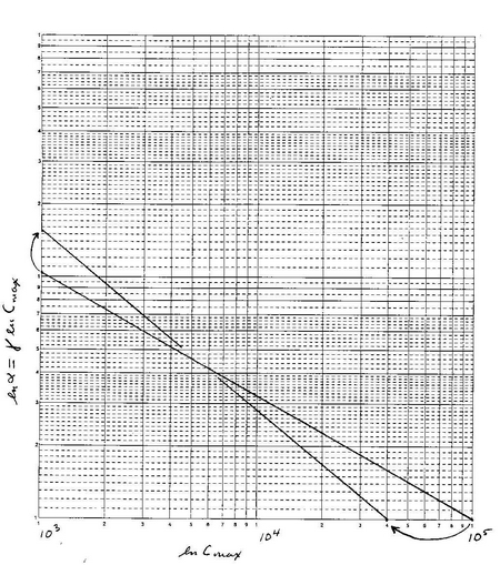
Each of the points on the world system trajectory represents a specific state of the world system as defined by F = αC-γ. If we consider a logarithmic plot of F = αC-γ, i.e. lnF = lnα – γlnC, the plot represents a triangular space on logarithmic axes bounded by the line represented by the previous equation and by the segment of the ordinate from ln 1 to γlnCmax and the segment of the abscissa from ln 1 to lnCmax. Note that as long as γ > 1 the bounding ordinate segment will be greater than the bounding segment of the abscissa. There are three ways to change the area of this triangle: 1. To change lnα (=γlnCmax). 2. To change lnCmax. (Any change in γ will automatically bring about a change in the magnitude of the bounding segment of the abscissa.) 3. To change both. As the world system moves along its trajectory, what is the strategy used? Which variable is changed, or is the mixed strategy employed, and, if so, what is the mixed strategy?
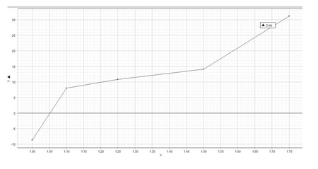
It will be instructive first to note the state of the world system as reflected by the relationship between α, Cmax, and γ at regular points over the five thousand year time span being investigated. In this instance one thousand year intervals have been chosen to reflect the broad trend of world system change (see Figure 12. The absolute value of the slope of each line is the value of γ as a consequence of the magnitude of both α and Cmax for that specific century. With the exception of the centuries 3000 BCE and 2000 BCE all sets of α, Cmax, and γ are unique. This of course implies that the position of the world system is unique and has evolved, i.e. changed, over time. Also, and not unexpectedly, as the world system progresses over the last five thousand years, there is an increase in the position of both intercepts, i.e. as both intercepts depend on the magnitude of the maximum urban area of a given point in time, Cmax, both intercepts increase as a consequence of the increased degree of urbanization over recorded history. However, while the degree of urbanization of the world system has increased over time, it has done so far from the point(s) of equilibria of that system, and in fact the world system is a non-equilibrium system.
If Eq. 18 is modified by multiplying through by C0, then this equation becomes, Cmaxγ – Cmax –(γ – 1)T = 0 (Eq. 24), and if this modified equation is then partially differentiated with respect to γ the partial derivative is: ∂f/ ∂γ = Cmaxγln Cmax – T. Further, by setting this partial derivative equal to zero and then solving for γ the following equation is produced: γ = [ln Cmax]-1ln[T/ln Cmax] (Eq. 25). This last equation gives the equilibrium value of γ, i.e. γeq, and can then be used to compute γeq for each value of Cmax and T per century over the period of time for which the world system is being analysed in this paper. Interestingly, when γeq is computed in this way, the values of γeq do not match γo, the observed values for gamma, but instead vary in a consistent and linear way from the observed value of gamma. The consistency of this difference is shown by regressing |γo – γeq|, ∆ γ, against γo, which gives: ∆γ = .257γo – .230 (Eq. 26.) and has an r-value of .992, which implies an exceptional fit. This relationship can be seen graphically in Figure 11. This then is one more line of evidence that suggests that the trajectory of the world system is constrained.
Figure 11.
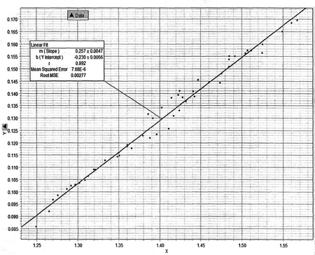
NOTES: The graph above represents the relationship between γo on the x-axis and ∆ γ on the y-axis. As can be seen by the linearity of the data and the value of r = .992, the data not only exhibit a linear trend but do so with very little dispersion about the line: ∆ γ = .257γo – .230. This implies significant constraint on the trajectory of the world system.
Unsurprisingly, if γeq is used to compute either the equilibrium value of Cmax or T, while using the observed value of the other variable, the magnitude of either varies consistently from the observed values of either. Specifically, when To, the observed value of the world system population, is compared with Teq, given that Teq can be computed by: Teq = [Cmaxγ – Cmax]/(γeq – 1), a linear regression of Teq v. To is produced, Teq = .3378 To – 6246618.955, and when the two sets of data, To and Teq, are compared using a 2-sample t-test the p-value is .1175, clearly indicating a difference in the two lists of data, To v. Teq. In a similar fashion using the observed value for T and the appropriate value for γeq and solving Eq. 24 for Cmax yields equilibrium values larger than the observed values, and these values vary systematically with observed values of Cmax. This is a consequence of the reduced value of γeq. The regression of Cmax(o) against Cmax(eq) yields: Cmax(eq) = 25.3 Cmax(o) – 1.02E+7 with an r value of .993, again an exceptionally close fit. The computed values of Cmax and T based on the equilibrium values of γ computed from Eq. 25 are significantly different than the values actually exhibited by the world system and clearly imply that the world system is a non-equilibrium system.
Since there is a consistent difference between observed and expected, i.e. equilibrium, values of γ and also between computed values of both Cmax and T, then, unquestionably, the world system is a non-equilibrium system, and it is appropriate to ask what factors are contributing to this consistent difference between observed values and predicted equilibrium values. Ball (2008) suggests that non-equilibrium systems are maintained away from equilibria by competing processes, and perhaps an extension of the current research would be to identify potential opposing processes and then assess their significance with respect to changes in gamma. For instance, the relationship between urbanization and de-urbanization or the relationship between technological innovation and carrying capacity might be worthy first choices, as would the cyclical nature of societal processes as demonstrated by Turchin and Nefedov (2009), although the significance of phase transitions that the world system has experienced in the past should also be considered in that whatever caused the phase transitions suggests an imbalance between those competing processes and may in fact make those processes more identifiable.
Even though a predictable difference exists between γo and γeq over the course of the last 5000 years Eq. 26 suggests that as γo decreases so does ∆γ, and since historically γo has decreased over the last 5000 years so also has done ∆γ. At what point will γo and γeq converge? This is easy enough to answer by setting Eq. 26 equal to zero. There is a convergence point between expected and observed γ when γo = γeq = .8949, and this convergence point is beyond the extinction point of γo = 1, i.e. when γo = 1, then Eq. 24 becomes: Cmax1 – Cmax – (1 – 1)T = 0, and this obviously holds for any values of Cmaxand T. In other words, at no time between 1 < γo ≤ 1.6 will the world system ever be at equilibrium, other than in the face of complete collapse. Also, as γo decreases the magnitude of the maximum urban area increases.
It will be instructive first to note the state of the world system as reflected by the relationship between α, Cmax, and γ at regular points over the five thousand year time span being investigated. In this instance one thousand year intervals have been chosen to reflect the broad trend of world system change (see Figure 12). The absolute value of the slope of each line is the value of γ as a consequence of the magnitude of both α and Cmax for that specific century. With the exception of the centuries 3000 BCE and 2000 BCE all sets of α, Cmax, and γ are unique. This of course implies that the position of the world system is unique and has evolved, i.e. changed, over time. Also, and not unexpectedly, as the world system progresses over the last five thousand years, there is an increase in the position of both intercepts, i.e. as both intercepts depend on the magnitude of the maximum urban area of a given point in time, Cmax, both intercepts increase as a consequence of the increased degree of urbanization over recorded history.
Even though the degree of urbanization has increased over time it has not done so in an even or constant rate. As mentioned previously the transition from 3000 BCE to 2000 BCE involved no net change in the magnitude of Cmax, and observation of all the time-incremented positions of the world system as represented in Figure 12 clearly show the influence, the uneven influence, of urbanization as represented by Cmax on the position of the world system has caused the progress(ion) of the world system itself to be uneven. First, γ is not constant over time but shows a broadly decreasing trend; this implies a greater proportional change in Cmax than in α. Over the last two thousand years there has been relatively little overall net change in γ, e.g. at 1 CE γ = 1.3090, at 1000 CE γ = 1.2969, and at 2000 CE γ = 1.2460. This also appears to be true of the period from 3000 BCE to 1000 BCE where at 3000 BCE γ = 1.4851, at 2000 BCE γ = 1.5640, and at 1000 BCE γ = 1.4756. The greatest change in γ occurred between 1000 BCE and 1 CE, i.e. from γ = 1.4756 to γ = 1.3090, a period of time encompassing Karl Jaspers' Axial Age.
Figure 12. The relationship, γ = lnα/lnCmax, represented at 1000 year intervals showing that the state of the world system changes so that the slope of the line increases, i.e. becomes less negative. This is due to changes in both lnα and lnCmax.
The actual position of the world system line is also not evenly spaced through time with the greatest difference represented by the transition from 1000 CE to 2000 CE. Unquestionably there are two distinctly different states of the world system represented on this graph and one period of transition. The first two thousand years are represented by a median value of γ = 1.5070 and the last 2000 years by a median value of γ = 1.2840. The middle one thousand years, the period of transition, has a median value of γ = 1.3923. It should be noted that the differences between the three medians is .1147 between the median of the first two thousand years and the middle one thousand years and is .1083 between the median of the middle one thousand years and the median of the final two thousand years. Quite obviously these differences are relatively close in magnitude suggesting changes of relative magnitude in the world system position.
In assessing the strategy used by the world system with respect to state space as defined previously several portions of the trajectory will be considered. These regions include portions of each search pattern, including sets of three data points increase in involving a decrease in γ and then an increase, a set that involves continuous increase in γ, another that involves continuous decrease in γ, and a set that involves a continuous increase from the first search pattern to the second.
Figures 13 and 14 represent increases in γ, while Figures 15 and 16 represent decreasing values of γ. In the case of Figures 13 and 14 the initial segments, from 3000 BCE to 2900 BCE and from 700 BCE to 600 BCE respectively, the change involved a decrease in γlnCmax and an increase in lnCmax, whereas in Figures 15 and 16, changes from 2300 BCE to 2200 BCE and 2100 BCE to 2000 BCE the reverse occurred; γlnCmax increased, and lnCmax decreased. In other words, when γ either increases or decreases both intercepts change but in the opposite direction, i.e. if γ decreases then γlnCmax decreases and lnCmax increases, while the reverse would be true if γ were to increase. Interestingly, the value of the partial derivative of lnF with respect to α decreases with increasing α, while the value of the partial derivative of lnF with respect to C increases with increasing C. So, increasing lnCmax while decreasing γlnCmax causes an increase in ∂lnF/∂α and a decrease in ∂lnF/∂C (see Figures 17 and 18).
Figure 13. This figure represents the change in the world system position as defined by γ, lnα, and Cmax from 700 BCE to 600 BCE. Note that γ increases as a function of both a decrease in lnα and an increase in Cmax.
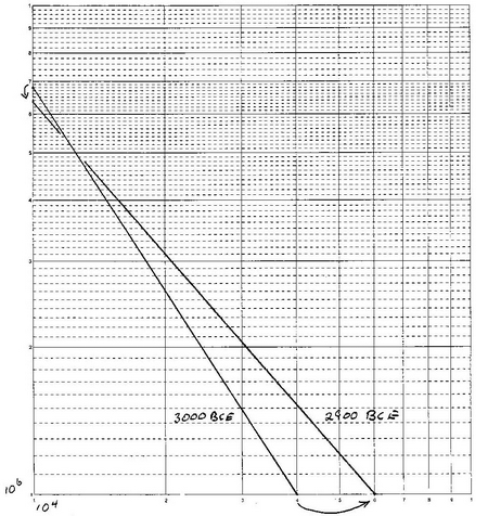
Figure 14. Here, as opposed to Figure 13, the change is reversed, and γ decreases as a function of increasing lnα and decreasing lnCmax. The period of time represented is the one hundred years intervening 2300 BCE and 2200 BCE.
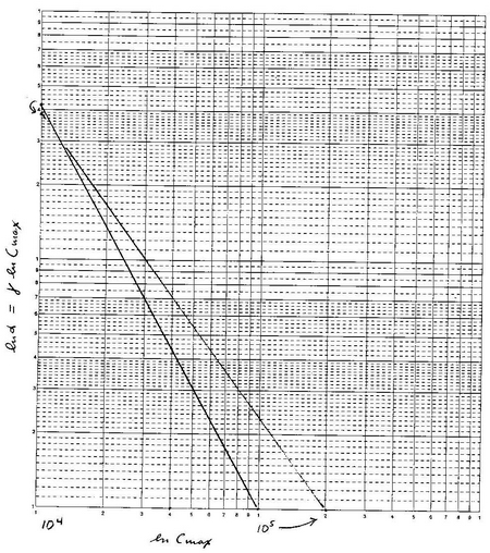
Figure 15. This figure represents the effects of a decrease in lnCmax as an attendant change to the increase of the absolute value of γ, which causes an increase in lnα during the century from 2300 BCE to 2200 BCE.
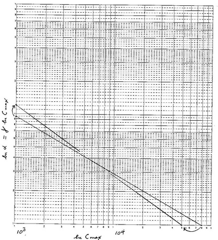
Figure 16. As in Figure 15 the absolute value of γ increases which causes similar changes in the state of the world system, i.e. a reduction in lnCmax which causes an increase in lnα, this time during the century from 2100 BCE to 2000 BCE.
In the case of continuous change with respect to the world system trajectory and considering the two sequences, 400 BCE to 100 BCE and 700 CE to 1000 CE, both representing continuous decreases in the magnitude of γ over a span of 300 years, it would be predicted that γlnCmax should decrease continuously while lnCmax should continuously increase, and this is exactly what is observed (see Figures 19 and 20). Specifically, for the period from 400 BCE to 100 BCE γlnCmax decreases from 21.97 to 20.31, while lnCmax increases from 12.68 to 13.82; in the period from 700 CE to 1000 CE, the same trends are observed as γlnCmax decreases from 22.10 to 20.95, while lnCmax increases from 12.90 to 14.00. It should be noted that there are fewer long term changes in which γ increases. However, if the period, 200 CE to 500 CE, is considered, the reverse trends would be predicted, i.e. an increase in γlnCmax with a concomitant decrease in lnCmax. In particular, γlnCmax increases form 20.40 to 21.61, and lnCmax decreases from 14.00 to 13.12. Again, observations match predictions (see Figure 21).
Figure 17. This figure represents the change in lnF with respect to α and is hyperbolic in form but always positive.
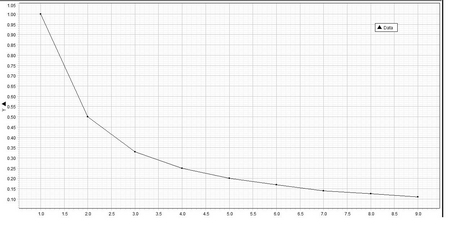
Figure 18. This graph indicates that as C increases so does the rate of change of lnF. However, the value of the rate of change in lnF is negative. This graph and the one in Figure 17 appear to be mirror images of one another, suggesting that as urbanization, as represented by Cmax, increases both partial differentials reduce in effect.
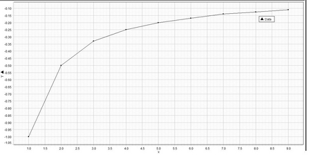
Figure 19. This graph represents the change in the world system over a period of 300 years, from 400 BCE to 100 BCE, in which the absolute value of γ continuously decreases. As a consequence there is a continuous increase in lnCmax and a decrease in γ lnCmax, which implies an increase in urbanization.
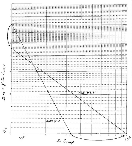
Figure 20. As in Figure 19 a continuous decrease in the absolute value of γ causes an increase in lnCmax and decreases γ lnCmax with the implication that the degree of urbanization increases during this period.
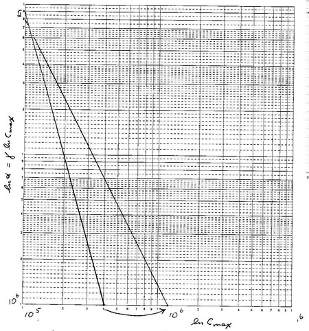
Figure 21. This graph represents the effects of a continuous increase in gamma had over the period, 200 CE to 500 CE. As expected, urbanization decreased, while the frequency of smaller communities increased.
At this point it is worth considering what the system would be like if the changes adopted by the world system were not of the mixed-strategy variety. What would it mean for γ to increase while keeping lnCmax constant? An increase in the value of γlnCmax would be required, and this implies an increase in the number of smaller urban areas. On the other hand if γlnCmax were to be held constant, then lnCmax would have to be decreased, and as this expression would automatically decrease with increasing γ, it is easier to understand this change within the context of a change in γ. However, all the evidence suggests that both intercepts change, and this may be an accommodation to the cost of changing the position of the world system. In other words, changing γ involves both a change in the size of urban areas and also a change in the frequency of urban area size classes. It should also be noted that much more time is spent in adjustment of both γlnCmax and lnCmax than in increasing population size. Why this should be is not obvious but probably involves adjusting to an optimal distribution of urban sizes and size distributions for a given global population size or, at least, global population size range.
While the rule of thumb with respect to the change in the positions of the abscissa and ordinate intercepts is that if Cmax or lnCmax, α and its log transform, lnα (=γlnCmax), increases, there are seven exceptions to this rule of thumb in which a decrease in γ, which is usually indicative of an increase in lnCmax and a consequent decrease in γlnCmax, is associated with an increase in γlnCmax or in one case where an increase in γ is associated with an increase in both lnCmax and logically γlnCmax. The following centuries are associated with an increase in γlnCmax and a decrease in γ: 900 BCE, 400 BCE, 600 CE, 1000 CE, 1900 CE, and 2000 CE, while 1800 CE shows an increase in γ, γlnCmax, and lnCmax.
It is interesting to consider what factors might be at play with regard to changes in γ and the attendant changes in lnCmax, and γlnCmax. That lnCmax increases as γ decreases is both logically predictable and empirically verifiable. A decrease in the absolute value of γ implies of course an increase in –γ, the implications of which are that the largest urban areas increase and the frequency of the smallest collective classes of people decreases. It is as if there is a pump that moves the populace of the world system from a less urbanized to a more urbanized condition. The inverse, when the absolute value of γ increases, population movement can be thought of as going in the reverse direction, with urbanization being associated with larger numbers of smaller individual urban areas. In circumstances in which both γlnCmax and lnCmax increase, the increase in urbanization must be relatively greater than the decrease in γ, but also there must be some synergy between smaller and larger urban areas.
Considering changes in γ alone, and defining γ as γ = lnα/lnCmax, allows dγ to be defined as dγ = 1/lnCmax – lnα/ln2Cmax. On the other hand when dγ is plotted against γ using the appropriate values of lnα and lnCmax, the graph (Figure 18) may be approximated as linear, and a regression of dγ on γ gives the equation: dγ = .135 – .113γ. Consequently, .135 – .113γ = 1/lnCmax – lnα/ln2Cmax, or (.135 – .113 γ)ln2Cmax – lnCmax + lnα = 0. This equation is a quadratic and may be solved using the quadratic formula. The solutions yielded give close approximations for lnCmax and consequently by transformation for Cmax. This indicates one more form of constraint on the system. It will now be revealing to consider the relationship between sequences of γ, i.e. γn, γn – 1, γn – 2, etc.
Of the three variables used to characterize the world system, as has been established previously, change in γ has the greatest effect on the system. In light of the importance of γ to the world system trajectory it will be important to investigate what the effects of current and past values of this variable will have on future values of the variable. This will be done graphically by investigating the graphs of γn+1: γn, γn+2: γn, and γn+3: γn. The relationship, γn+1: γn, will be investigated first.
In Figure 22 γn is represented on the x-axis and γn+1 is represented on the y-axis. With five significant exceptions the trend exhibited by this plot is linear and represented by the regression, γn+1 = .866γn + .2197. The five outliers, numbered 1 through 5 on Figure 22, represent the following centuries: (1) 2000 BCE, (2) 2200 BCE, (3) 2100 BCE, (4) 1900 BCE, and (5) 2000 CE. The first three points represent a period of time, 2200 BCE to 2000 BCE, during which the Early Bronze Age experienced considerable climatic, economic, and social change. There are a number of instances in which societal collapse occurred during this time, e.g. the Akkadian Empire, the Old Egyptian Empire, and a number of smaller city states such as that found at Tel Leilan, and the Indus Civilization. The last two outlying points represent the last two hundred years of the world system trajectory. Removal of these outliers from the data set gives a linear regression of: γn+1 = .847γn + .2562, which is not significantly different from the previous regression.
Figure 22. γn, x-axis, is plotted against γn+1, y-axis, in this graph revealing a linear distribution of points with several notable outliers.
The implication of this regression is that there is a clear linear trend exhibited by the plot of the total population of points, in other words, that γn+1 depends on γn in a simple, proportional fashion. However, if the sequence by which the space of the plot in Figure 22 is traced chronologically, then the actual relationship, γn+1: γn, is not linear. In fact, the space, when critical points are removed resembles a parabola and potentially may indicate a chaotic system, although this point has yet to be confirmed (Figure 22).
When considering the relationship between γn and γn+2, the relationship is unquestionably linear, but with greater dispersion of points (see Figure 23). It should be noted that the overall shape of this distribution is dumbbell-like, and it should also be noted that this shape is a precursor of the distribution determined by γn+3: γn. The chronological sequence by which the space defined by γn+2: γn is not as revealing as that defined by γn+1: γn.
Figure 23. In this figure γn, x-axis, is plotted against γn+2, y-axis. In this graph, while the primary distribution is linear, there is a clear separation of two distinct clusters, to the right side of the graph one associated with the Ancient World, and one to the left associated with the Classical and Modern Worlds.
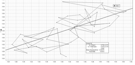
Figure 24. This graph shows clearly that, as with the previous plots, the distribution of points is essentially linear. However, since γn, x-axis, is plotted against γn+3, y-axis, there is an even more distinct separation between the Ancient World on the right hand side of the graph and that of both the Classical and Modern worlds on the left than in Figure 23. Also note that the transition between these two clusters of points occurs with an initially increasing value of the γ:γn+3 which moves the graph down and to the right. A similar trend occurs with the last three plots ending with the value of γ for 2000 CE.
In Figure 24 above, the plot of γn+3: γn, there are two discrete distributions of points and a shared unoccupied region between the two. The larger cluster is bounded by 1.37 ≤ γn ≤ 1.57 and for γn+3 the range is 1.39 – 1.57, approximately the same, and the lower cluster of points is bounded by 1.27 ≤ γn ≤ 1.42 and 1.24 ≤ γn+3 ≤ 1.42. The unoccupied region of overlap is bounded in the following way: 1.38 ≤ γn ≤ 1.42 and 1.32 ≤ γn+3 ≤ 1.45. The implications of the first and third distributions are significant in that they imply limits on the values of γn adopted by the world system as it evolves over time. If γn falls within the bounds, 1.38 – 1.42 then γn+3, a value of γ characteristic of the world system three hundred years on, cannot fall within the bounds, 1.38–1.45. This condition places limits on the direction of the world system trajectory and suggests that the world system is not only limited by sequential values of γbut also by values of γseparated by 300 years! Further, the transition from the first, older cluster to the second and younger cluster had to involve considerable change in γover that three hundred year period. For example, (1) is the last point in the upper, older cluster, and point (2) is the first in the lower cluster. (1) has the co-ordinates, 1.43 at 600 BCE and 1.36 at 300 BCE, and amounts to a change in γof –.07. (2) has the co-ordinates, 1.42 at 400 BCE and 1.27 at 100 BCE, amounting to a change in γof –.15. Note also that the changes from 600 BCE to 400 BCE and from 300 BCE to 100 BCE are respectively –.01 and –.09. These values are all great enough to bridge the gap described previously. The gap itself may signify a clear difference between the Ancient World and the Classical World with respect to the parameters, γ, a, and T, and is suggestive of a difference in organization and probably reflects differences in technology, communication, and intellectual paradigms to suggest just three, that separates the Ancient World from the Classical World. It is worthwhile indicating here that points (3) and (4) represent the most recent past and the time that we are in currently and may be (are) harbingers of a revolutionary change in the position of the world system from its current trajectory. Is the world system entering another period of search pattern behavior? Time will tell.
As has been previously mentioned the world system has two broadly different aspects to its trajectory, periods of continuous change punctuated by periods termed search patterns. A casual inspection of Figures 3, 4, and 5 will show that even though these different aspects occur at different orders of magnitude with respect to a and T, to the eye they appear within the context of mental scaling to be of the same magnitude. In more formal terms in any of the two-dimensional logarithmic plots the distance between any two consecutively chronological plots at one order of magnitude is within an order of magnitude of the distance between two consecutive points at a different order of magnitude. This casual inspection suggests self-similarity of world system behavior and that, as conjectured earlier in this paper, the world system behavior represented by the original equation, F = αC-γ, is scale-free.
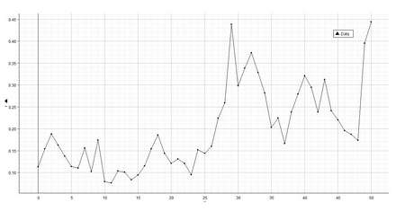
In order to demonstrate this, the actual distances between points in Figure 8b were calculated by using the Pythagorean theorem here represented by the equation: H = [(a1 – a0)2 + (T1 – T0)2]1/2. (Note: The value for a0 used to calculate H is always the initial value at 3000 BCE.) The magnitude of H was then divided by either the corresponding Cmax or T values, and these scale-normalized values of H were then plotted against time over the five thousand year range of the data on these variables. This gives the plot in Figure 25.
Figure 25. This graph represents a time series of the normalized changes in position of the world system per century over the last five thousand years. Normalization was done by dividing the change in position of the world system, a distance computed by Pythagorean Theorem, by the size of the maximum urban area of the current century. See text for explanation. Of significance is the very obvious periodicity of the world system trajectory when represented this way.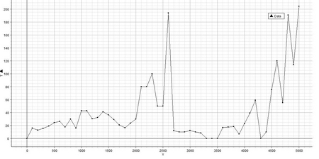
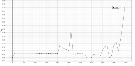
Figure 26. This graph reveals the same pattern as in Figure 25. However, the change in world system position was normalized by dividing the change in position of the world system by the total population of the system.
There are two aspects of this graph that are striking. First there appears to be a repeated pattern, quasi-periodic, with a period of about 1400 years. Second, the world system behavior represented by this graph shows steep descent from the peak at 400 BCE, and it is tempting to speculate that the world system will experience another precipitous change in position within the next one hundred years or so based upon the current position of the world system.
It is also important to note that embedded within this graph are the basic features of Modelski's world system graph of world cities and global population. Note that at 1000 BCE as with 1000 CE the world system begins a steep climb which terminates about 1000 years afterwards. In other words, Modelski's Ages of Reorganization are represented in this graph by periods of time when there is reduced magnitude of H/Cmax, and the Ages of Growth in Modelski's model correspond to periods of increased magnitude of H/Cmax. There are also some other interesting features of this graph. There are periods of relatively little change in H/Cmax such as from 300 CE to 500 CE, and there are periods of constant change as characterized by the period from 100 BCE to 200 CE, where H changes is very little and consequently the position of the world system is relatively static. Finally and most importantly, the plots of both H/Cmax and H/T exhibit similar but not identical trends, with the magnitude of the trends being greater for H/Cmax, possibly implying that the trajectory of the system is more sensitive to changes in Cmax than it is to T. In light of the previously demonstrated inequality, ∂f/∂γ > ∂f/∂a > ∂f/∂T, this should not be surprising as a = Cmax/C0.
It has been previously established that γ is the most influential variable on the trajectory of the world system. Since the trajectory of the world system, when normalized to either Cmax or T exhibits a similar and periodic behavior over the 5000 year period analysed it will be important to consider the relationship between Cmax and γ and T and γ. To some extent this has already been done in an earlier portion of this segment of the paper, and at this point it will be briefly treated with respect to the similarity between the two regressions. However, a linear regression of the natural log-transformed data on both Cmax and T with respect to γ may be used to compare the influences of the two variables on γ and those regressions may also be used to investigate secondary trends not apparent in the original data.
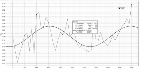
A linear regression of lnT on γ was calculated giving Eq. 24: γ = 3.7736 – .1106T, and this equation was used to generate expected values for γ per T. The residuals of each pair of values, observed minus expected, were computed and plotted against time to give the graph in Figure 27. Note that while this graph exhibits considerable variation there is a clear sinusoidal trend over the time period represented of 5000 years. Beyond this broad general trend there are several significant troughs that correspond to historically documented events. These are the Early Bronze Age Collapse occurring between 2200 BCE and 2000 BCE, the European Dark Age from approximately 400 CE to 800 CE, and the Plague Centuries from 1200 CE to 1400 CE. While it is important that the negative residuals correspond to collapse-related events, the inverse seems not to apply, since the fluorescence of a society occurs over a significant period of time. It is interesting to note that the period of time over which the Roman Empire became a world power is represented on the graph by a steep decline. This is also the period of time occupied by the Han Dynasty in China, the Kushan state in northern India, and the Sassanid Persians, and it is also a time during which an incipient Silk Road began functioning. That the temporal pattern of residuals over time does not specifically match specific and significant historical events should not be considered a weakness of the data, as the data represent global changes in γ, T, and a and are therefore system averages.
The program, Data Studio, was used to generate not only the plot in Figure 27 but also to generate best-fit circular functions to this data. In Figure 28 a sine curve is fitted to the data having an RMSE of .0874. The world system trajectory can then be represented by the equation, R = asin(bT + c) + d, where a, b, c, and d are fitted constants. The visual fit of the sine curve to the distribution of residuals is distinct, and the period of this fitted curve is 3740 years. Also, both florescences and declines of societies occurring during both the crests and troughs, e.g. the Late Bronze Age Collapse is associated with a crest, while, again, the rise of Rome is associated with a trough. As a final note, we in the Twenty-first Century occupy a position on the second crest of this sinusoidal trend of the world system and are in the process of transitioning to the descending side of this curve.
Figure 27. This figure represents a graph of the residuals of the Eq. 24 and exhibits a cyclical pattern which is formally defined by the next graph.
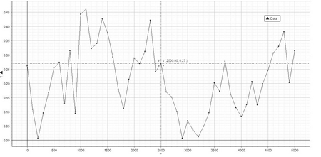
Figure 28. The cyclical nature of this plot is represented by the equation, R = asin(bT + c) + d, in which R, the value of the residuals, is represented on the y-axis.
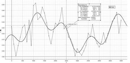
If a sine-series fit on this data (see Figure 29) is used instead of a sine fit, then the equation generated has the form: R = a0sin[(b0T)/1050 + c0] + d0 + + a1[(b1T)/525 + c1] + d1 and the resulting curve, while it exhibits an overall sinusoidal form, has multiple peaks and troughs, three per period, and an RMSE of .0708 suggesting a slightly better fit than the sine function alone. The period of this more complex sine-series curve is 3800 years. However, since this curve gives a slightly more accurate fit, the Late Bronze Age Collapse is now associated with a minor trough as are the European Dark Age and the Plague Century.
Figure 29. This is a sine-series fit to the residuals of Eq. 24, is a better fit than the sine fit of Figure 28.
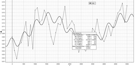
The same type of analysis can be performed on the relationship, lna on γ, which produces similar results (see Figure 30). However, while the sine fit gives a predictable curve with a different period, 3280 years as opposed to 3740 years. Also, the sine-series fit produces a different type of curve (see Figure 31). These differences can be attributed to the differences between the process of urbanization and that of global population growth, and it is important to recognize that these curves are out of phase with the process of urbanization occurring with a shorter period than that of global growth.
Figure 30. This graph is of the residuals of lna with respect to gamma over time and has the same general form as the graph in Figure 27 with some minor differences. These differences, however, do manifest themselves in a different sine-series fit than in Figure 29. See Figure 31.
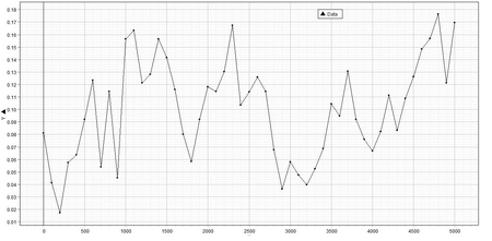
Figure 31. A sine-series fit of the data represented in Figure 30 is given here. Clearly, while this fit gives a closer approximation to the events represented, there is much that is not coincident with this fit, e.g. the significant troughs toward the end of both the Early and Late Bronze Ages.
Summary
The intent of this paper is to present a means of representing the trajectory of the world system over the last 5000 years. This is done by first constructing a mathematical model based on the assumption that urban area distribution in any given time period can be represented by F = αC-γ (Eq. 1). The model based on this assumption, aγ C0γ – 1 – a – (γ – 1)T/ C0 = 0 (Eq. 18), permits both the construction of a theoretical landscape, which represents all possible states of the world system and also the actual path of the world system based on values of γ, lna, and lnT. The general morphology of the theoretical landscape is one of a mostly flat plane which slopes upward as γ decreases and both lna and lnT increase. The theoretical landscape has a critical edge at γ = 0, as at that value the equation equals zero regardless of the values of either a or T. It is within this framework, this standard of comparison that the actual position and trajectory of the world system is analysed.
It was discovered, by analysing the variables in a pair-wise fashion, i.e. lna v. γ, lnT v. γ, and lnT v. lna, that in the instances where both lna and lnT are plotted against γ, these relationships are inverse, while lnT v. lna is a directly proportional and effectively linear relationship. However, within these broad trends there are two sub-trends that are unsurprisingly common to all three plots. These are periods of oscillation punctuated by periods of continuous, directed growth. The oscillatory periods are labeled search-patterns due to their apparent searching for the appropriate state of the world system that will then allow continuous, directed change over several centuries. There are two broad periods of these search-patterns, one encompassing the time period associated with most of the Ancient World, 2700 BCE to about 600 BCE, and the other from 100 BCE to 1800 CE, which includes much of the Classical World, the Middle Ages, the Renaissance, and the Modern World to 1800 CE. It should be noted here that more could be made of the fine structure of these periods, however that is not the focus of this paper.
Both search-pattern periods are defined in terms of their graphical position with no special regard to specific historical events. It was previously pointed out that both search-patterns include periods of collapse and the attendant Dark Ages or Ages of Reorganization to these periods of collapse. While the search-patterns are characteristic of all plots, it is noted that changes in γ are associated with almost no change in the magnitude of lnT, but as γ decreases in absolute value a lna increases and vice versa. As was mentioned previously the relationship between lnT and lna is direct and can be represented by the linear equation, lnT = .873 lna + 11.500.
There are a number of important implications of these major trends which are characteristic of the world system trajectory. Clearly, urbanization is associated with increases in global population, and, in fact, T is probably dependent on urbanization for its increase. An important consequence of this dependency is that the fraction of non-urban or rural population decreases over time as is represented by the equation: Tu/Tr = (a1-γ – 1)/(1 – C0γ-1) (Eq. 23). Another important consequence of the world system trajectory is that it occupies very little of the theoretical landscape delineated earlier.
The chief components affecting the position of the world system within the theoretical space defined are the relative effects of changing γ, a, and T on Eq. 18. It is shown that changing γ as represented by the partial derivative, ∂f/∂γ, has the greatest influence on the world system trajectory. The implications of this are far reaching. Since γ is a measure of the distribution of urban areas and is also a proxy for world system connectedness, periods of change in γ represent periods of change in the distribution of urban areas and consequently in their connectedness. Increases in γ, i.e. in the absolute value of γ, affect the distribution so that there are fewer urban areas with high populations and many more with lower populations. This is a process of de-urbanization, increasing ruralization, and reduced connectedness within the world system. The reverse holds for decreasing values of γ; these periods represent increasing urbanization and greater connectedness.
Change in the world system may be represented in a variety of ways. The natural log transform of Eq. 1 gives lnF = lnα – γlnCmax, and for appropriate values of α and Cmax then it is shown that γ = lnα/lnCmax, and per century the state of the world system may be represented graphically by the triangular area bounded by the natural log transform of Eq. 1 and the x-axis and y-axis intercepts. Given this graphical representation then the change in the state of the world system can be represented by changes in lnα, lnCmax, or both, a mixed strategy in other words. It can be shown that when γ decreases lnα decreases and lnCmax increases, however when γ increases, the reverse occurs. In other words and even in the face of increasing population, T, changes in γ are associated with a mixed strategy employing change in both lnα and lnCmax. One anomaly has been noted, that of the change associated with the change in the state of the world system from 1300 CE to 1400 CE where both intercepts increase. Excluding this anomalous instance unquestionably the mixed strategy imposes a constraint on the trajectory of the world system.
That the world system has a trajectory suggests that past conditions of the world system influence its future position. This effect was investigated by considering plots of γn+1 v. γn, γn+2 v. γn, and γn+3 v. γn. As might be expected the plot of γn+1 v. γn is essentially linear, however the plots, γn+2 v. γn, and γn+3 v. γn, reveal that the data cluster into two discrete sets implying a boundary condition between the Ancient and Classical World on the one hand and the Medieval and Modern ones on the other. The influence of the magnitude of γ two and three centuries later suggests a clear and probably qualitative difference between the two sets of points. Further, the transition from the older set of points to the set including the current world system suggests a unique pathway between those two sets.
Observation of the plots, lna v. γ, and lnT v. γ reveals a repeating pattern of oscillations punctuated by continuous change. If the distance in theoretical space over which the world system moves from century to century is scaled by dividing by either lna or lnT the graph of these scaled distances over time reveals a cyclical trend with an approximate period of 2400 years giving peaks at 400 BCE and 2000 CE. Both plots give similar patterns in which the largest shifts of the world system are succeeded by periods of relative stasis that extend over several centuries. It appears that we are currently on the doorstep of such a period.
The relationship of γ v. lnT was investigated to reveal any secondary trends as was the relationship, γ v. lna. The residuals of both regressions revealed similar cyclical trends which were then fitted to both sine and sine-series functions. The periodicity of these trends ranged from approximately 3300 years to 3800 years. The sine function fit of the γ v. lnT data gives a period of 3700 +/–210 years with peaks in the middle of the second millennium BCE and now and troughs at the beginning of the Bronze Age and the time of Late Antiquity. However, this general fit does not account for many of the smaller troughs and peaks in the residual-generated graph, e.g. a trough at the end of the Early Bronze Age and a peak at approximately 700 CE are associated respectively with a peak and a trough of the actual sine function. These and other details are not reflected in the sine fit. The sine-series fit of the same data give better but not complete resolution suggesting that these trends are predictable.
The same sets of trends are observable in both the sine and sine-series fit of the residuals of γ v. lna linear regression. The periods for these fits are respectively 3280 +/–220 years and 3290 +/–210 years. It is noted however that while the overall trends represented by both sine and sine-series fit are similar, due to differences in periodicity, the curves themselves are offset. Since the periods are not similar, the interrelationship of the urbanization and total world system population size is not a directly interactive one as is, say, the relationship between predator and prey.
In brief then the following statements may be made about the trajectory of the world system over the last 5000 years:
1. With respect to the variables, γ, lna, and lnT, the world system clearly exhibits a non-random pattern or trajectory over the last 5000 years.
2. In pair-wise analysis of the variable listed in No. 1 similar patterns emerge, but with respect to γ in relation to either lna or lnT the relation is inverse, while the relation between lna and lnT is direct.
3. The world system exhibits periods of oscillation punctuated by periods of continuous change, the latter always being associated with a decrease in the absolute value of γ.
4. Change in the magnitude of γ has the greatest influence on the state and direction of the world system trajectory.
5. The world system is a non-equilibrium system.
6. In natural log phase space the world system can be represented as an area bounded by lnF = lnα – γlnCmax, and a change in the nature of this phase space involves a mixed strategy of changing both the x-axis and y-axis intercepts, lnCmax and lnα. There is at least one exception to this strategy, that of the transition from 1300 CE to 1400 CE.
7. The magnitude of γ is influenced by prior values of this variable, and the graph of γ separated by three centuries on itself reveals a clear separation between the (relatively) Modern World and the Classical and Ancient Worlds.
8. The behavior of the world system, as measured by distance moved per century, is shown to be similar at different orders of magnitude scaled by both lna and lnT. Specifically, a repeating pattern is evident in which large movements of the world system within the theoretical space defined by Eq. 18 are succeeded by periods of near stasis.
9. The greatest change in γ occurs between 1000 BCE and 1 CE.
10. Residuals of the linear regression of lna v. γ and lnT v. γ reveal cyclical patterns that can be modeled by both sine and sine-series functions. The curves produced by these functions are faithful to and coincident with a number of major historical events including but not limited to various age-terminating collapses.
Mathematical appendix
Derivation of equation 18
The total population of the world system, T, is then the sum of the world system urban population Tu, and that portion of the population existing rurally, Tr. Each of these is an integral of F, however, by modifying the integral of the total population an expression can be derived that will permit T, a, the ratio of the largest urban area to the smallest urban area, and γ, as defined previously, to be inter-related:
T = ∫F = α∫C-γdC, (Eq. 2)
but with different limits. Tu has the limits, C0 to Cmax,, where these limits represent the smallest and largest urban, and the definite integral has the form:
Tu = [α/(1 – γ)][Cmax1 – γ – 1]. (Eq. 3)
Tr has the limits, 1 to C0, and the definite integral is:
Tr = [α/(1 – γ)][ C01 – γ – 1]. (Eq. 4)
Note that Cmax can be expressed as a function of C0 in that Cmax is a multiple of C0 and can be represented by:
Cmax = aC0, (Eq. 5)
where a is some real number greater than zero. Also note that, assuming that there can theoretically be a single largest urban area, then Eq. 1 can be rewritten as:
1 = αCmax-γ. (Eq. 6)
It follows then that:
α = Cmaxγ. (Eq. 7)
In turn and according to Eq. 4, Eq. 6 may be rewritten as:
α = aγC0γ. (Eq. 8)
So, then substituting into Eq. 3 gives:
Tu = [aγC0γ /(1 – γ)][ a1 - γC01 – γ – C01 – γ], (Eq. 9)
and further simplifying gives:
Tu = [aγC0γ C01 – γ/(1 – γ)][ a1 - γ – 1], (Eq. 10)
which may be further simplified to:
Tu = [aγC0/(1 – γ)][ a1 - γ – 1]. (Eq. 11)
By the same reasoning then Tr may be represented as:
Tr = [aγC0/(1 – γ)][1 – C0γ – 1]. (Eq. 12)
Since
T = Tu + Tr, (Eq. 13)
then by substitution:
T = [aγC0/(1 – γ)][ a1 - γ – 1] + [aγC0/(1 – γ)][1 – C0γ – 1]. (Eq. 14)
Further rearrangement gives:
T = [C0/(1 – γ)][a – aγ] + [aγC0/(1 – γ)] [1 – C0γ – 1], (Eq. 15)
then by further rearrangement:
T = aC0/(1 – γ) – aγ C0/(1 – γ) + aγC0/(1 – γ) – aγC0γ/(1 – γ). (Eq. 16)
Noticing that the second and third terms cancel and multiplying through by (1 – γ)/ C0 gives:
(1 – γ)/ C0T = a – aγ C0γ – 1, (Eq. 17)
and a final rearrangement gives:
aγ C0γ – 1 – a – (γ – 1)T/ C0 = 0. (Eq. 18)*
* Please note that the same equation could be derived directly by integrating over the limits, 1 to Cmax, however, it was felt that by doing a piece-meal integration, it would be easier to understand where urbanization fits into the larger context of the total world system population. Also, it is understood that the distribution represented by Eq. 1, F = αC-γ, implies that the largest class, i.e. the class with the highest frequency, would be individuals living alone. This is clearly not the case, however, in this paper this inadequacy of the model will be ignored.
Derivation of equation 23
Recalling that Cmax = aC0, that α = Cmaxγ, and that Tu = α∫C-γdC over the limits C0 to Cmax, then the evaluation of this integral is:
Tu = [(aγC0γ)/(1 – γ)][ Cmax1-γ – C0γ-1], (Eq. 19)
which simplifies to:
Tu = [(aγC0γ)/(1 – γ)] [a1-γC01-γ – C01-γ], (Eq. 20)
and further simplifies to:
Tu = [(aγC0)/(1 – γ)] [a1-γ – 1]. (Eq. 21)
Using the same reasoning the integral, Tr, can be evaluated over the limits, 1 to C0, as:
Tr = [(aγC0)/(1 – γ)] [1 – C0γ-1]. (Eq. 22)
Since the term, [(aγC0)/(1 – γ)], is common to both Eq. 21 and Eq. 22, the ratio, Tu/Tr, becomes:
Tu/Tr = (a1-γ – 1)/(1 – C0γ-1). (Eq. 23)
Tables
|
CENTURY |
SEQUENCE |
T |
Cmax |
a |
γO |
|
1 |
2 |
3 |
4 |
5 |
6 |
|
3000 BCE |
0 |
14E6 |
40E3 |
4E2 |
1.4851 |
|
2900 |
100 |
14.95E6 |
60E3 |
6E2 |
1.4245 |
|
2800 |
200 |
15.97E6 |
80E3 |
8E2 |
1.3859 |
|
2700 |
300 |
17.05E6 |
70E3 |
7E2 |
1.4145 |
|
2600 |
400 |
18.21E6 |
60E3 |
6E2 |
1.4470 |
|
2500 |
500 |
19.44E6 |
50E3 |
5E2 |
1.4847 |
|
2400 |
600 |
20.76E6 |
50E3 |
5E2 |
1.4921 |
|
2300 |
700 |
22.17E6 |
80E3 |
8E2 |
1.4227 |
|
2200 |
800 |
23.68E6 |
50E3 |
5E2 |
1.5070 |
|
2100 |
900 |
25.29E6 |
10E4 |
1E3 |
1.4024 |
|
2000 |
1000 |
27E6 |
40E3 |
4E2 |
1.5604 |
|
1900 |
1100 |
28.72E6 |
40E3 |
4E2 |
1.5674 |
|
1800 |
1200 |
30.54E6 |
60E3 |
6E2 |
1.5047 |
|
1700 |
1300 |
32.49E6 |
60E3 |
6E2 |
1.5115 |
|
1600 |
1400 |
34.55E6 |
50E3* |
5E2 |
1.5491 |
|
1 |
2 |
3 |
4 |
5 |
6 |
|
1500 |
1500 |
36.74E6 |
60E3 |
6E2 |
1.5250 |
|
1400 |
1600 |
39.08E6 |
80E3 |
8E2 |
1.4846 |
|
1300 |
1700 |
41.56E6 |
12E4 |
1.2E3 |
1.4280 |
|
1200 |
1800 |
44.20E6 |
16E4 |
1.6E3 |
1.3917 |
|
1100 |
1900 |
47.01E6 |
12E4 |
1.2E3 |
1.4410 |
|
1000 |
2000 |
50E6 |
10E4 |
1E3 |
1.4756 |
|
900 |
2100 |
60E6 |
12.5E4 |
1.25E3 |
1.4603 |
|
800 |
2200 |
70E6 |
12.5E4 |
1.25E3 |
1.4763 |
|
700 |
2300 |
80E6 |
10E4 |
1E3 |
1.5248 |
|
600 |
2400 |
90E6 |
20E4 |
2E3 |
1.4322 |
|
500 |
2500 |
10E7 |
20E4 |
2E3 |
1.4428 |
|
400 |
2600 |
16.2E7 |
32E4 |
3.2E3 |
1.4239 |
|
300 |
2700 |
15.6E7 |
50E4 |
5E3 |
1.3606 |
|
200 |
2800 |
15E7 |
60E4 |
6E3 |
1.3333 |
|
100 |
2900 |
16E7 |
10E5 |
1E4 |
1.2757 |
|
1 CE |
3000 |
17E7 |
80E4 |
8E3 |
1.3090 |
|
100 |
3100 |
18E7 |
10E5 |
1E4 |
1.2869 |
|
200 |
3200 |
19E7 |
12E5 |
1.2E4 |
1.2699 |
|
300 |
3300 |
19E7 |
10E5 |
1E4 |
1.2920 |
|
400 |
3400 |
19E7 |
80E4 |
8E3 |
1.3195 |
|
500 |
3500 |
19E7 |
50E4 |
5E3 |
1.3793 |
|
600 |
3600 |
20E7 |
60E4 |
6E3 |
1.3606 |
|
700 |
3700 |
20.7E7 |
40E4 |
4E3 |
1.4170 |
|
800 |
3800 |
22E7 |
70E4 |
7E3 |
1.3499 |
|
900 |
3900 |
22.6E7 |
90E4 |
9E3 |
1.3211 |
|
1000 |
4000 |
25.4E7 |
12E5 |
1.2E4 |
1.2969 |
|
1100 |
4100 |
30.1E7 |
12E5 |
1.2E4 |
1.3125 |
|
1200 |
4200 |
36E7 |
10E5 |
1E4 |
1.3508 |
|
1300 |
4300 |
36E7 |
15E5 |
1.5E4 |
1.3022 |
|
1400 |
4400 |
35E7 |
10E5 |
1E4 |
1.3483 |
|
1500 |
4500 |
42.5E7 |
10E5 |
1E4 |
1.3657 |
|
1600 |
4600 |
54.5E7 |
10E5 |
1E4 |
1.3879 |
|
1700 |
4700 |
60E7 |
10E5 |
1E4 |
1.3963 |
|
1800 |
4800 |
81.3E7 |
11E5 |
1.1E4 |
1.4112 |
|
1900 |
4900 |
15.5E8 |
65E5 |
6.5E4 |
1.2654 |
|
2000 |
5000 |
62E8 |
23E6 |
2.3E5 |
1.2490 |
Partial Derivative Table
|
T |
T/C0 |
γ |
a |
∂f/∂ γ |
∂f/∂a |
|
106 |
104 |
1.00 |
400 |
–5761 |
0 |
|
“ |
“ |
1.1 |
“ |
2987 |
3 |
|
“ |
“ |
1.25 |
“ |
49944 |
17 |
|
“ |
“ |
1.50 |
“ |
1317048 |
299 |
|
“ |
“ |
1.75 |
“ |
3.5E13 |
4949 |
|
“ |
“ |
1.25 |
400 |
49944 |
17 |
|
“ |
“ |
1.25 |
4000 |
1287592 |
30 |
|
“ |
“ |
1.25 |
12000 |
5549521 |
40 |
|
“ |
“ |
1.25 |
24000 |
13867614 |
48 |
The following equations were used to calculate the values listed in the Partial Derivative Table: aγ C0 γ – 1 – a – (γ -1)T/C0 = 0, ∂f/∂ γ = aγln(a) + aγ C0 γ – 1ln C0 – T/C0, ∂f/∂a = γaγ – 1 C0 γ – 1 – 1 .
Acknowledgements
I wish to acknowledge the following people for their help and counsel: Prof. Dmitri Bondarenko, Prof. Leonid Grinin, Prof. Andrey Korotayev, Sherry Donovan, Paul Kim, Mary Lappan, David Reinstein, Sarah Kapnick, Prof. Peter Turchin, and Lauren Dickey. I wish to give special thanks to Boris Spektor without whose technical assistance this paper would not have been possible. I also wish to thank Kseniya Biryukova for her excellent editorial assistance. While all made significant contributions to this work, I alone accept full responsibility for any errors.
Bibliography
Ball, P. 2009. Branches. Natures Patterns: A Tapestry in Three Parts. New York: Oxford University Press.
Chandler, T. 1987. Four Thousand Years of Urban Growth. New York: Edwin Mellen Press.
Diakonov, I. M. 1999. The Paths of History. New York: Cambridge University Press.
Frank, A. G., and W. R. Thompson. 2005. Afro-Eurasian Bronze Age Economic Expansion and Contraction Revisited. Journal of World History 16(2): 115–172.
Jaspers, K. 1965. The Origin and Goal of History. New Haven: Yale University Press.
Korotayev, A., and L. Grinin. 2006. Urbanization and Political Development of the World System: A Comparative Quantitative Analysis. History and Mathematics. Historical Dynamics and Development of Complex Societies / Ed. by P. Turchin, L. Grinin, A. Korotayev, V. de Munck, pp. 115–153. Moscow: KomKniga/URSS.
Korotayev, A., and D. Khaltourina. 2006. Introduction to Social Macrodynamics: Secular Cycles and Millennial Trends in Africa. Moscow: URSS.
Korotayev, A., A. Malkov, and D. Khaltourina. 2006a. Introduction to Social Macrodynamics: Compact Macromodels of the World System Growth. Moscow: URSS.
Korotayev, A., A. Malkov, and D. Khaltourina. 2006b. Introduction to Social Macrodynamics: Secular Cycles and Millennial Trends. Moscow: URSS.
Marx, K. 1977. A Contribution to the Critique of Political Economy. Moscow: Progress Publishers.
Modelski, G. 2003. World Cities: –3000 to 2000. New York: Faros.
Raup, D. M., and A. Michelson. 1965. Theoretical Morphology of the Coiled Shell. Science 3663: 1294–1295.
Toynbee, A. 1946. A Study of History. New York: Oxford University Press.
Turchin, P. 2003. Historical Dynamics: Why States Rise and Fall. Princeton: Princeton University Press.
Turchin, P., and S. A. Nefedov. 2009. Secular Cycles. Princeton, NJ: Princeton University Press.
Wallerstein, I. 1974. The Modern World System. New York: Academic Press.
Wallerstein, I. 2004. World System Analysis: An Introduction. Durham, NC: Duke University Press.
[1] Note that the exponent, γ, is a logarithm.